Excel determines that rows meet the requirements

excel determines that rows meet the requirements

Insert the command button in Sheet2 and program it as follows:

Private Sub CommandButton1_Click()

Dim i1 As Long, i2 As Long

Dim a$, b$

i2 = 2

Do While Range(＂C＂ & i2) ＂＂"

a$ = ＂＂

b$ = ＂＂

i1 = 1

Do While Worksheets(＂Sheet1＂).Range(＂C＂ & i1) ＂＂"

If Worksheets("sheet1").Range("C" & i1) = Range("C" & i2) Then

a$ = a$ & Worksheets(＂sheet1＂).Range(＂A＂ & i1) & ＂;＂

b$ = b$ & Worksheets(＂sheet1＂).Range(＂B＂ & i1) & ＂;＂

End If

i1 = i1 1

Loop

If a$ "＂ Then a$ = Left(a$, Len(a$) - 1)

If b$ ＂＂ Then b$ = Left(b$, Len(b$) - 1)

Range(＂A＂& i2) = a$

Range(＂B＂& i2) = b$

i2 = i2 1

Loop

End Sub

How to get the several lines of text before and after a specific string under Linux

This line of command can help you delete the commit block containing Merge (any multiple such text blocks)

sed -n '/commit/{:a;h;n;/Merge/b;:c;H;n;$bd;/commit/!bc;:d;x;p;x;ba} ' log > log.txt

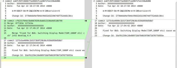
The operation effect is as follows:

My command may be a bit complicated. A little explanation, just for reference:

Where: a :b :c :d is the command jump label label

1. /commit/{:a;h;n;

When a commit is found on a line, copy this line to the hold space, and then read the next line.

2. /Merge/b;

If the new line just read contains Merge, end the processing of this line, read the next line, and continue to look for commit

If the new line just read does not contain Merge, then continue to execute subsequent commands on this line:

3. :c;H;n;$bd;/commit/!bc;:d;x;p;x;ba}

Append this line to the hold space and read the next line. If the last line is not reached and commit is not found, execute the command bc and jump to the c label - loop this process until the end of the file is read or Read the line containing commit. Then, x, swaps the content of the hold space with the content of the pattern space, p, outputs the content of the pattern space (that is, the block that does not contain the Merge), x, swaps it again, and the pattern space becomes the previous content (the end of the file or contains commit line). ba, jump to label a, continue checking this line, and repeat steps 1, 2, and 3.

If the above command is changed to:

sed -n '/commit/{:a;h;n;/Merge/!b;:c;H;n;$bd;/commit/!bc;:d;x;p;x;ba }' log > log.txt

Then, the output result is, only the commit block containing Merge

Read the data and number of rows and columns in the TXT file in MFC

Since there are 1-digit data and 4-digit data, if there is no special carriage return in the txt, the number of rows and columns cannot be determined. If there is a carriage return, simply use

#include

char *strtok( char *str1, const char *str2 );

can be solved.

First use getline() to read a str per line, and accumulate the number of lines, then

char *result = NULL;

char string[100][100];

int x = 0;

result = strtok( str, " ");

while( result != NULL ) {

strcpy(string[x] , result);

result = strtok( NULL, " " );

}

In this way, all data can be saved using a string array. x records the total number, and then x divided by the number of rows is the number of columns.

I’m free today, and I’ll help you write out the entire program:

#include

#include

#include

using namespace std;

void main(){

char ch[100] = "\0";

char b[100][100];

int x=0,y=0;

ifstream fin(＂123.txt＂,ios::in);

fin.getline(ch,100);

while(!fin.eof()){

x;

cout

char *result = NULL;

result = strtok(ch,＂,＂);

while( result != NULL ) {

strcpy(b[y ],result);

cout

result = strtok( NULL, ＂,＂ );

}

memset(ch,0,100);

fin.getline(ch,100);

}

fin.close();

}

//It has been run before, no problem, b[100][100] is all elements, x is the number of rows, y/x is the number of columns.

The above is the detailed content of Excel determines that rows meet the requirements. For more information, please follow other related articles on the PHP Chinese website!