You Need to Know What the Hash Sign Does in Excel Formulas

Excel Overflow Range Operator (#) allows formulas to be automatically adjusted to accommodate changes in overflow range size. This feature is only available for Microsoft 365 Excel for Windows or Mac. Common functions such as UNIQUE , COUNTIF , and SORTBY can be used in conjunction with overflow range operators to generate dynamic sortable lists.

The pound sign (#) in the Excel formula is also called the overflow range operator, which instructs the program to consider all results in the overflow range. Therefore, even if the overflow range increases or decreases, the formula containing # will automatically reflect this change.

How to list and sort unique values ​​and text in Microsoft Excel

Use simple functions to create a list of unique names, dates, or other data in a spreadsheet.

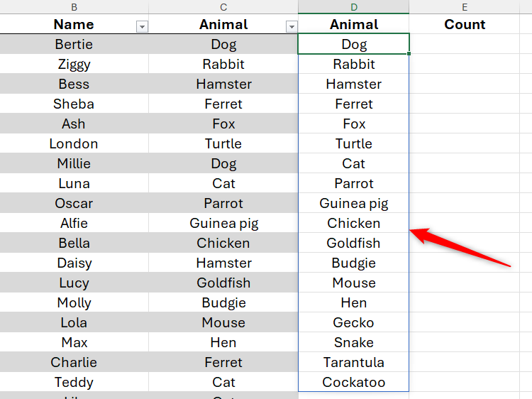
Example After pressing Enter, you will get an overflow array listing each unique item in the Animal column. When you select any affected cells, the blue border shows that the area is an overflow array.

All you need to know about overflowing in Excel

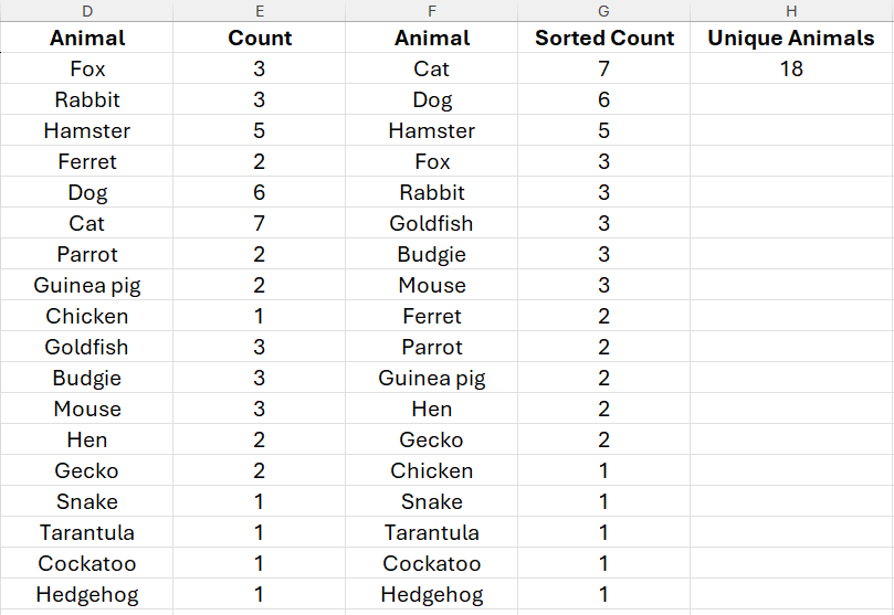
Now, let's calculate the number of each animal in the table, using the pound mark makes the operation much easier.

To do this, you need to use the COUNTIF function. However, in order for Excel to count all animals returned by the UNIQUE function in column D (even if some animals are added or removed to this list later), you need to add a pound sign after the conditional reference.

Therefore, in cell E2, type:

 <code>=COUNTIF(Animals_Admitted[Animal],D2#)</code>

Among them, COUNTIF is a function that calculates the number of occurrences, Animals_Admitted[Animal] is the range that contains each animal in the original table. D2# tells Excel that the condition of the COUNTIF function is an overflow array starting from cell D2, so the size may change.

The example assumes that the turtle is released in London. After removing London from the original data (it is the only turtle in the shelter), cell H2 correctly shows that you now have only 18 unique animals and the turtle no longer appears in the other list you created.

Overflow range operator (#): Final prompt

Before you start, you need to pay attention to the following points:

First, in addition to referring to overflow ranges in the same worksheet, you can also reference overflow ranges in another worksheet. For example, to reference an overflow array starting from cell A2 in worksheet 2, you can type:

 <code>=Sheet2!A1#</code>

Second, you can reference the overflow range in another workbook. Although Microsoft pointed out that the referenced workbook must be open to avoid returning a #REF! error, in my tests, the reference still worked even if the workbook is closed. Just make sure you save both workbooks and connect them both to the same OneDrive account to ensure that no data is lost.

Finally, to avoid the formula returning a #SPILL! error, make sure that all cells that the array is going to overflow have no other data and are not merged.

---

Whether you want to extend your understanding of Excel formulas and functions, or apply for jobs that require Excel expertise, you can confidently say that you know the role of pound signs in Microsoft Excel formulas!

The above is the detailed content of You Need to Know What the Hash Sign Does in Excel Formulas. For more information, please follow other related articles on the PHP Chinese website!