
 Software Tutorial
Office Software
Use the PERCENTOF Function to Simplify Percentage Calculations in Excel
Software Tutorial
Office Software
Use the PERCENTOF Function to Simplify Percentage Calculations in Excel
Use the PERCENTOF Function to Simplify Percentage Calculations in Excel

Excel's PERCENTOF function: Easily calculate the proportion of data subsets
Excel's PERCENTOF function can quickly calculate the proportion of data subsets in the entire data set, avoiding the hassle of creating complex formulas.
PERCENTOF function syntax
The PERCENTOF function has two parameters:
<code>=PERCENTOF(a,b)</code>
in:
- a (required) is a subset of data that forms part of the entire data set;
- b (required) is the entire dataset.
In other words, the PERCENTOF function calculates the percentage of the subset a to the total dataset b .
Calculate the proportion of individual values using PERCENTOF
The easiest way to use the PERCENTOF function is to calculate the proportion of a single value in the sum.
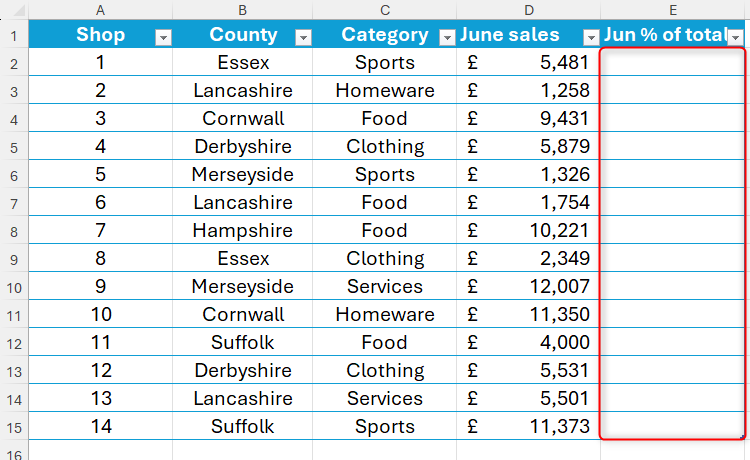
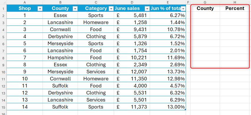
For example, analyze the performance of 14 stores in England in June and calculate the contribution of each store to total sales for the month.
This example uses formatted Excel tables and structured references to make the formula easier to understand. If more data is added on line 16 and below, the new value will be automatically included in the calculation. If you do not use tables and structured references, you may need to adjust the formula to include absolute references and update the formula when adding more data rows.
Enter in cell E2:
<code>=PERCENTOF(</code>
Then click on cell D2 (the subset of data to calculate its contribution to the sum). If formatted tables are used, this forces Excel to add column names to the formula, while the @ symbol indicates that each row will be considered separately in the result. Then add a comma:
<code>=PERCENTOF([@[June sales]],</code>
Finally, select all the data in column D (including the data subset selected in the previous step, but not the column header), telling Excel which cells make up the entire dataset. This will be displayed in the formula as the column name in square brackets. Then close the original parentheses.
<code>=PERCENTOF([@[June sales]],[June sales])</code>
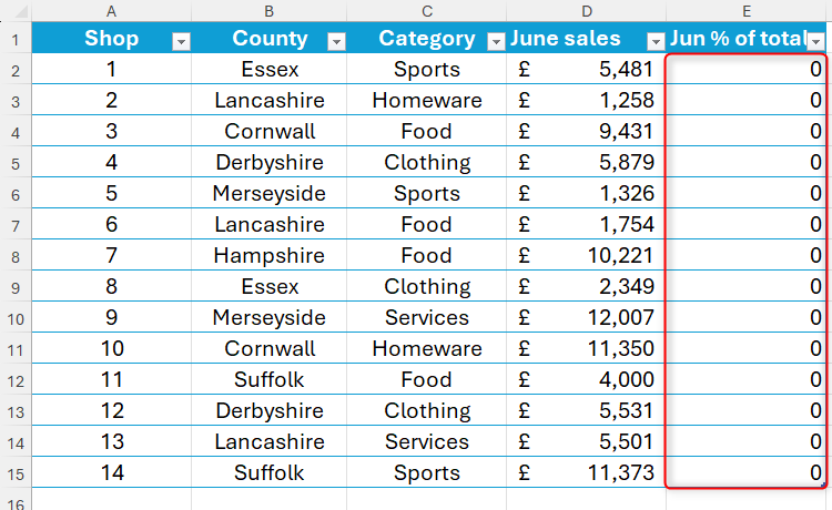
After pressing Enter, the result will be displayed as a series of zeros. Don't worry, this is because the data in the percentage column is currently expressed as a decimal, not a percentage.
To change these values from a decimal to a percentage, select all affected cells and click the % icon in the Numbers group of the Ribbon Start tab. Meanwhile, click the "Increase Decimals" button to add decimals, which will help distinguish similar values.
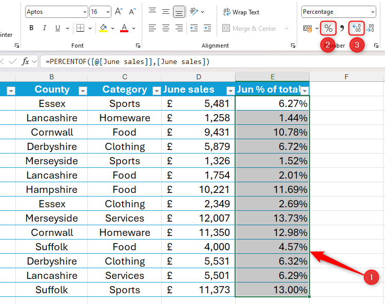
This gives a formatted Excel table with a column showing how each store contributes to total sales.
Related content##### Excel’s 12 digital format options and their impact on data
Adjust the number format of the cell to match its data type.
using PERCENTOF with GROUPBY
While PERCENTOF can be used alone to display individual percentage contributions, it is mainly added to Excel for use with other functions. Specifically, PERCENTOF works very well with GROUPBY, and you can further subdivide the data into specified categories and display the output as a percentage.
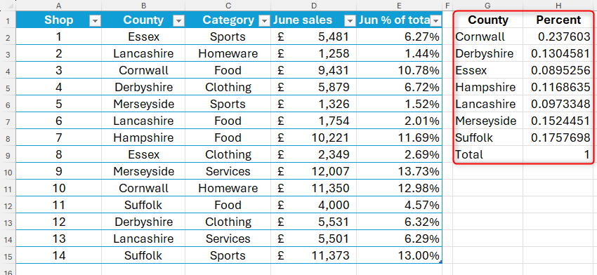
Keep using the store sales data example above, assuming the goal is to find out which counties attract the largest percentage of sales.
Because GROUPBY creates dynamic arrays, this function cannot be used in formatted Excel tables. This is why you need to create a data retrieval form in a spreadsheet area that is not formatted as a table.
To do this, enter:
<code>=GROUPBY(Sales[County],Sales[June sales],PERCENTOF)</code>
in:
- Sales[County] is the field in the original Sales table that will determine the grouping;
- Sales[June sales] is a field containing the value that will generate the percentage;
- PERCENTOF is a function that converts raw data into comparison values.

Related content##### How to name tables in Microsoft Excel
"Table1" is not explained clearly enough...
GROUPBY function also allows input of five additional optional fields such as field title, sort order, and filter array, but in this case these fields are omitted to show how to use them with PERCENTOF in the simplest form.
After pressing Enter, Excel will group sales by county (alphabetical by default), displaying data in decimals.
To convert these decimals into percentages, select these numbers and click the % icon in the Numbers group of the Start tab of the ribbon. You can also adjust the decimal places of a percentage number by clicking the "Increase Decimal places" or "Decimal places" buttons in the same tab group.
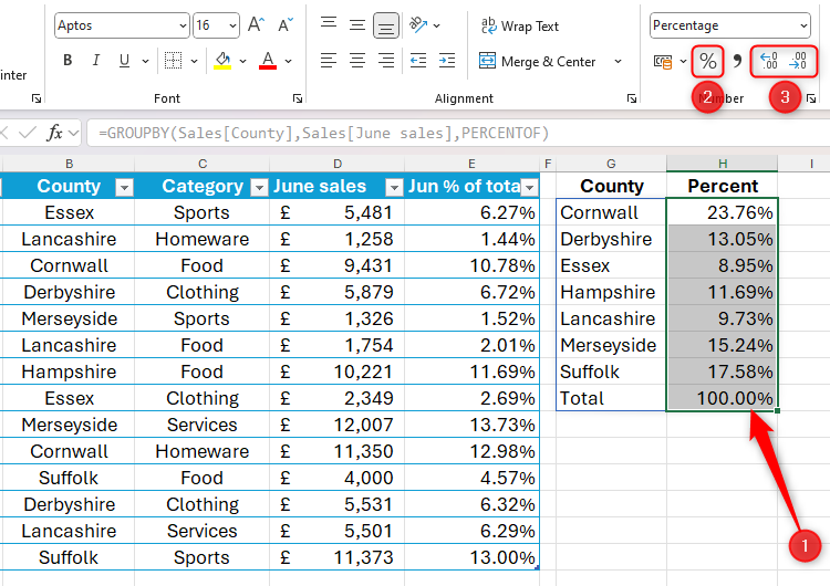
Now, even if the data changes dramatically, the GROUPBY function picks up these changes and adjusts the classification table accordingly.
The application of PERCENTOF is much more than that! For example, you can embed this function in PIVOTBY, further segment the data using multiple variables, and then display the output as a percentage.
The above is the detailed content of Use the PERCENTOF Function to Simplify Percentage Calculations in Excel. For more information, please follow other related articles on the PHP Chinese website!

Hot AI Tools

Undresser.AI Undress
AI-powered app for creating realistic nude photos

AI Clothes Remover
Online AI tool for removing clothes from photos.

Undress AI Tool
Undress images for free

Clothoff.io
AI clothes remover

Video Face Swap
Swap faces in any video effortlessly with our completely free AI face swap tool!

Hot Article
Hot Tools

Notepad++7.3.1
Easy-to-use and free code editor

SublimeText3 Chinese version
Chinese version, very easy to use

Zend Studio 13.0.1
Powerful PHP integrated development environment

Dreamweaver CS6
Visual web development tools

SublimeText3 Mac version
God-level code editing software (SublimeText3)
Hot Topics


 How to Create a Timeline Filter in Excel
Apr 03, 2025 am 03:51 AM
How to Create a Timeline Filter in Excel
Apr 03, 2025 am 03:51 AM
In Excel, using the timeline filter can display data by time period more efficiently, which is more convenient than using the filter button. The Timeline is a dynamic filtering option that allows you to quickly display data for a single date, month, quarter, or year. Step 1: Convert data to pivot table First, convert the original Excel data into a pivot table. Select any cell in the data table (formatted or not) and click PivotTable on the Insert tab of the ribbon. Related: How to Create Pivot Tables in Microsoft Excel Don't be intimidated by the pivot table! We will teach you basic skills that you can master in minutes. Related Articles In the dialog box, make sure the entire data range is selected (
 If You Don't Use Excel's Hidden Camera Tool, You're Missing a Trick
Mar 25, 2025 am 02:48 AM
If You Don't Use Excel's Hidden Camera Tool, You're Missing a Trick
Mar 25, 2025 am 02:48 AM
Quick Links Why Use the Camera Tool?
 You Need to Know What the Hash Sign Does in Excel Formulas
Apr 08, 2025 am 12:55 AM
You Need to Know What the Hash Sign Does in Excel Formulas
Apr 08, 2025 am 12:55 AM
Excel Overflow Range Operator (#) enables formulas to be automatically adjusted to accommodate changes in overflow range size. This feature is only available for Microsoft 365 Excel for Windows or Mac. Common functions such as UNIQUE, COUNTIF, and SORTBY can be used in conjunction with overflow range operators to generate dynamic sortable lists. The pound sign (#) in the Excel formula is also called the overflow range operator, which instructs the program to consider all results in the overflow range. Therefore, even if the overflow range increases or decreases, the formula containing # will automatically reflect this change. How to list and sort unique values in Microsoft Excel
 Use the PERCENTOF Function to Simplify Percentage Calculations in Excel
Mar 27, 2025 am 03:03 AM
Use the PERCENTOF Function to Simplify Percentage Calculations in Excel
Mar 27, 2025 am 03:03 AM
Excel's PERCENTOF function: Easily calculate the proportion of data subsets Excel's PERCENTOF function can quickly calculate the proportion of data subsets in the entire data set, avoiding the hassle of creating complex formulas. PERCENTOF function syntax The PERCENTOF function has two parameters: =PERCENTOF(a,b) in: a (required) is a subset of data that forms part of the entire data set; b (required) is the entire dataset. In other words, the PERCENTOF function calculates the percentage of the subset a to the total dataset b. Calculate the proportion of individual values using PERCENTOF The easiest way to use the PERCENTOF function is to calculate the single
 If You Don't Rename Tables in Excel, Today's the Day to Start
Apr 15, 2025 am 12:58 AM
If You Don't Rename Tables in Excel, Today's the Day to Start
Apr 15, 2025 am 12:58 AM
Quick link Why should tables be named in Excel How to name a table in Excel Excel table naming rules and techniques By default, tables in Excel are named Table1, Table2, Table3, and so on. However, you don't have to stick to these tags. In fact, it would be better if you don't! In this quick guide, I will explain why you should always rename tables in Excel and show you how to do this. Why should tables be named in Excel While it may take some time to develop the habit of naming tables in Excel (if you don't usually do this), the following reasons illustrate today
 How to Format a Spilled Array in Excel
Apr 10, 2025 pm 12:01 PM
How to Format a Spilled Array in Excel
Apr 10, 2025 pm 12:01 PM
Use formula conditional formatting to handle overflow arrays in Excel Direct formatting of overflow arrays in Excel can cause problems, especially when the data shape or size changes. Formula-based conditional formatting rules allow automatic formatting to be adjusted when data parameters change. Adding a dollar sign ($) before a column reference applies a rule to all rows in the data. In Excel, you can apply direct formatting to the values or background of a cell to make the spreadsheet easier to read. However, when an Excel formula returns a set of values (called overflow arrays), applying direct formatting will cause problems if the size or shape of the data changes. Suppose you have this spreadsheet with overflow results from the PIVOTBY formula,

 How to Use Excel's AGGREGATE Function to Refine Calculations
Apr 12, 2025 am 12:54 AM
How to Use Excel's AGGREGATE Function to Refine Calculations
Apr 12, 2025 am 12:54 AM
Quick Links The AGGREGATE Syntax
