Two modes of Excel 'read-only mode'

php editor Xiaoxin introduces to you the "read-only mode" in Excel, which is a mode that prevents others from changing the content of the file. In Excel, there are two read-only modes to choose from, namely "Protect Sheet" and "Open as Read-Only". These two modes can help users effectively protect file contents, prevent accidental modification or deletion, improve work efficiency and ensure data security.

"Read-only mode" 1:

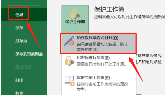
After opening the Excel table, click the [File] menu, select [Information] → [Protect Workbook] → [Always open in read-only mode]. After saving the file, the "read-only mode" setting is completed.

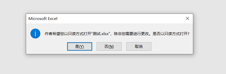
Open the Excel table again, and a dialog box will pop up, prompting "Unless you need to make changes, do you want to open it in read-only mode?", select "Yes", the table will be opened in "read-only mode"; select "No", After the form is opened, it can be edited and modified normally.

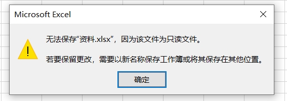
If you accidentally modify and save an Excel table opened in "read-only mode", a prompt will pop up indicating that the file cannot be saved. If you want to save it, you need to rename it to a new file before saving it.

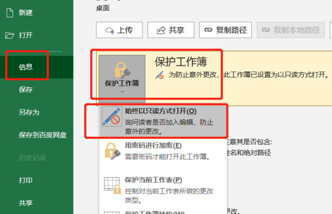
If you want to cancel "read-only mode", when you need to open Excel, select "No" under the option "Whether to open in read-only mode" and enter Excel in normal editing mode before you can cancel.

Then follow the set operation process, that is, click [File] → [Information] → [Protect Workbook] → [Always open as read-only], then save the file, and Excel’s “read-only mode” will be lifted. .

"Read-only mode" 2:

In method 1, you can freely choose whether to open the Excel table in "read-only mode". Next, we will introduce another "read-only mode", which requires a password to be edited normally.

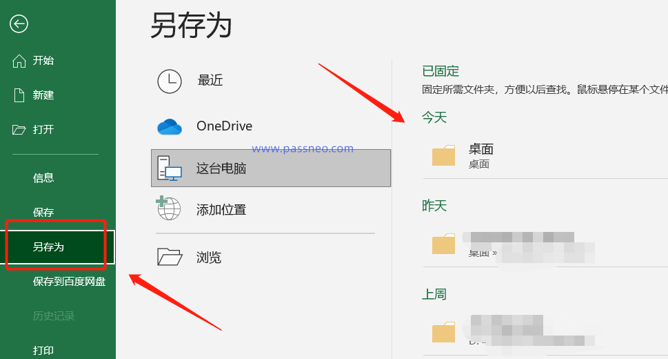
After opening the Excel table, also click the [File] option in the menu list, then click [Save As] in the new page, and determine the saving directory after saving on the right;

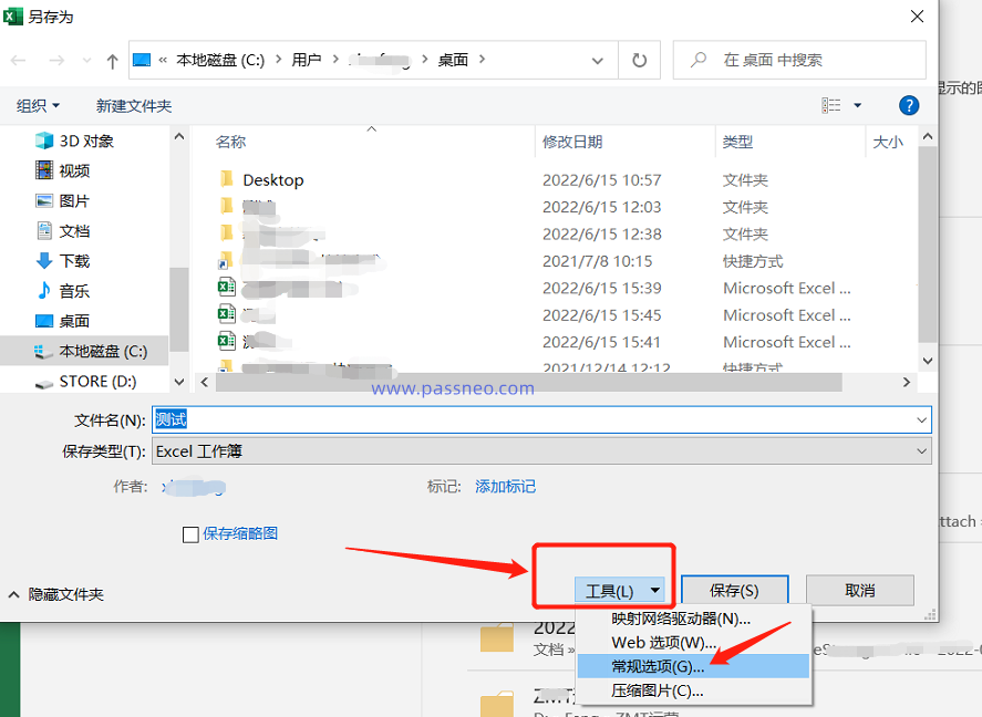
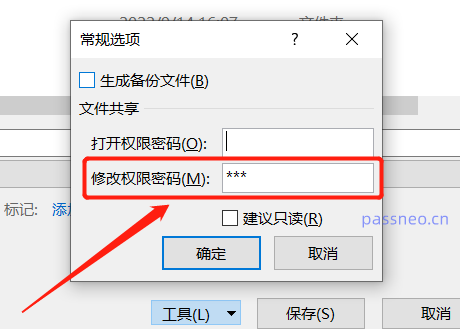
After the [Save As] dialog box pops up, click [General Options] in the [Tools] option below;

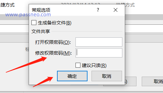
After the dialog box pops up, enter the password you want to set in the [Modify Permission Password] column, and then re-enter the password; after clicking [OK], you can change the name and save it as a new file, or you can directly replace the original file. . After saving, the "read-only mode" of Excel is set.

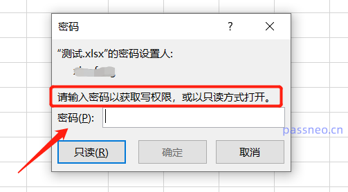
Open the Excel table again, and a prompt box will also pop up. If you select "Read-only", the file will be opened in "read-only mode". If you want to edit normally, you need to enter the originally set password.

It should be noted that although the Excel table in "Method 2" requires a password to be edited normally, after opening it in "Read-only mode", just like "Method 1", the content can still be modified. After modification The original Excel cannot be saved, but it can be saved by changing the name and saving it as a new Excel.

How to cancel "read-only mode 2"?

After opening the Excel table, enter the password, open the file for normal editing, and then follow the set operations, select [File] → [Save As] → “Select Save Directory” → [Tools] → [General Options], and then The existing password in the [Modify Permission Password] column is cleared. After saving the file, the "read-only mode" of Excel is released.

In addition to using the above method to cancel the "read-only mode" of the Excel table, we can also use tools to directly remove the "read-only mode".

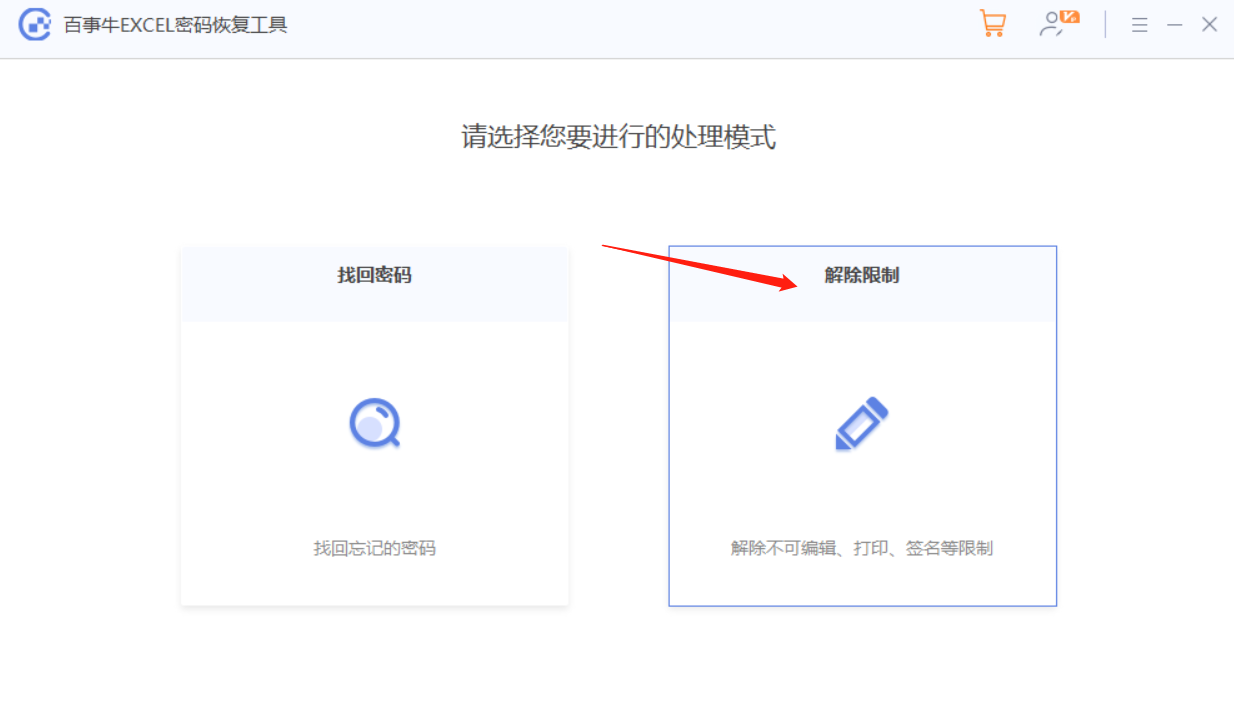
Take the Pepsi Niu Excel password recovery tool as an example. It can not only remove the "read-only mode" of the Excel table with one click, but also remove the "restricted editing" that requires a password to lift. It is a tool worth collecting.

Regardless of whether the Excel table is set to "read-only mode" or "restricted editing", click the [Unrestriction] module in the tool and then import the Excel table to remove it directly.

Tool link: Pepsi Niu Excel Password Recovery Tool

The above is the detailed content of Two modes of Excel 'read-only mode'. For more information, please follow other related articles on the PHP Chinese website!