

Macro that splits an Excel sheet into 300 rows per sheet

A macro that divides an excel sheet into one sheet every 300 rows!
Public Sub mySub()
Dim shS As Worksheet: Set shS = ActiveSheet 'Source data sheet, current active sheet
Dim rS&: rS = 1 'Source data table, start reading data from this row
Dim rC&: rC = 300 'The number of rows read each time
Dim rNew$: rNew = 1 'Create a new table and paste the data into this row
Dim rZ&: rZ = shS.UsedRange.Row shS.UsedRange.Rows.Count - 1
Dim shNew As Worksheet, nm$, n%, r&
r = rS
Do While r
n = n 1
Set shNew = Worksheets.Add(after:=Sheets(Worksheets.Count))
nm = "Table" & rC & "_"" & n
Call ShNm(shNew, nm)
shS.Rows(r).Resize(rC).Copy shNew.Rows(rNew)
r = rC * n rS
Loop
MsgBox "ok"
End Sub
Public Sub ShNm(sh As Worksheet, nm As Variant)
On Error Resume Next
100:
sh.Name = nm
If Err.Number 0 Then
Err.Clear
nm = Application.InputBox( _
" " " & nm & " " already exists! " & Chr(10) & Chr(10) & "Please enter a new table name: ", _
"Please enter the new table name", nm & "_new", _
Type:=2)
If nm = False Then MsgBox "The input is incorrect, exit the program!": End
GoTo 100
End If
End Sub
How to use macro commands to split a sequence in EXCEL, for example, split PL10 120 into
Sub Macro6()
'
' Macro6 Macro
'
'
Selection.TextToColumns Destination:=Range("A1"), DataType:=xlDelimited, _
TextQualifier:=xlDoubleQuote, ConsecutiveDelimiter:=False, Tab:=False, _
Semicolon:=False, Comma:=False, Space:=False, Other:=True, OtherChar _
:="*", FieldInfo:=Array(Array(1, 1), Array(2, 1)), TrailingMinusNumbers:=True
Columns("A:A").Select
Selection.Replace What:="PL", Replacement:="", LookAt:=xlPart, _
SearchOrder:=xlByRows, MatchCase:=False, SearchFormat:=False, _
ReplaceFormat:=False
Columns("C:D").Select
Selection.Insert Shift:=xlToRight, CopyOrigin:=xlFormatFromLeftOrAbove
Range("C1").Select
ActiveCell.FormulaR1C1 = "=MIN(RC[-2],)"
Range("C1").Select
ActiveCell.FormulaR1C1 = "=MIN(RC[-2],RC[-1])"
Range("D1").Select
ActiveCell.FormulaR1C1 = "=MAX(RC[-3],RC[-2])"
Range("C1:D1").Select
Selection.AutoFill Destination:=Range("C1:D1000")
Range("C:D").Select
Columns("A:B").Select
Range("B1").Activate
Columns("C:D").Select
Selection.Copy
Selection.PasteSpecial Paste:=xlPasteValues, Operation:=xlNone, SkipBlanks _
:=False, Transpose:=False
Columns("A:B").Select
Range("B1").Activate
Application.CutCopyMode = False
Selection.Delete Shift:=xlToLeft
Columns("A:B").Select
Selection.Replace What:="0", Replacement:="", LookAt:=xlWhole, _
_
SearchOrder:=xlByRows, MatchCase:=False, SearchFormat:=False, _
ReplaceFormat:=False
End Sub
Note: When using it, select column A first and then run the macro. The column to be split must be in column A, and the two columns BC are empty, otherwise it will be overwritten (haha, the time is short, not particularly smart) and the number of rows No more than 1000 lines. Haha, otherwise it will be a bit slow, so the range is set at 1000 lines. Are you also engaged in steel structures? Haha, too
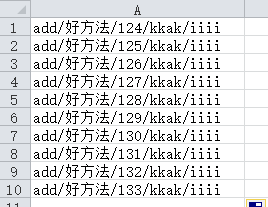
How to use macros in EXCEL to split the automatic symbols with A and these in the table into the following columns
Option Explicit
Sub test()
Dim rng As Range
Dim arr As Variant
Dim k As Integer
For Each rng In Selection
rng.Value = Replace(rng.Value, ":", "/")
arr = Split(rng.Value, "/")
k = UBound(arr) 1
rng.Resize(1, k) = arr
Erase arr
Next rng
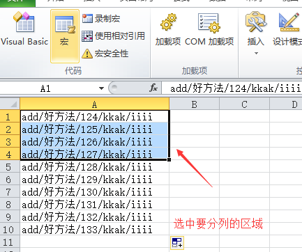
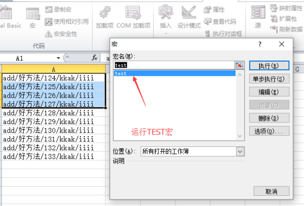
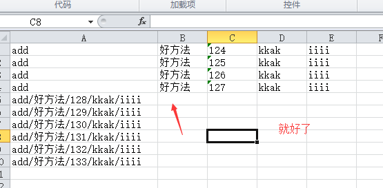
End Sub I think you know how to paste the code, so I won’t go into details. Just press the image below to run the code I wrote for you:
step-1
step-2
step-3
step-4
How to quickly split an excel table into multiple excel tables and retain the original formulas
Click [Development Tools]-[Visual Basic] or the Alt F11 shortcut key to enter the VBE editing interface.
Choose to insert a new module
Paste the following code into the module:
Sub CFGZB()
Dim myRange As Variant
Dim myArray
Dim titleRange As Range
Dim title As String
Dim columnNum As Integer
myRange = Application.InputBox(prompt:="Please select the title row:", Type:=8)
myArray = WorksheetFunction.Transpose(myRange)
Set titleRange = Application.InputBox(prompt:="Please select the split header, which must be the first row and be a cell, such as: "Name"", Type:=8)
title = titleRange.Value
The above is the detailed content of Macro that splits an Excel sheet into 300 rows per sheet. For more information, please follow other related articles on the PHP Chinese website!

Hot AI Tools

Undresser.AI Undress
AI-powered app for creating realistic nude photos

AI Clothes Remover
Online AI tool for removing clothes from photos.

Undress AI Tool
Undress images for free

Clothoff.io
AI clothes remover

Video Face Swap
Swap faces in any video effortlessly with our completely free AI face swap tool!

Hot Article
Hot Tools

Notepad++7.3.1
Easy-to-use and free code editor

SublimeText3 Chinese version
Chinese version, very easy to use

Zend Studio 13.0.1
Powerful PHP integrated development environment

Dreamweaver CS6
Visual web development tools

SublimeText3 Mac version
God-level code editing software (SublimeText3)
Hot Topics


 How to Create a Timeline Filter in Excel
Apr 03, 2025 am 03:51 AM
How to Create a Timeline Filter in Excel
Apr 03, 2025 am 03:51 AM
In Excel, using the timeline filter can display data by time period more efficiently, which is more convenient than using the filter button. The Timeline is a dynamic filtering option that allows you to quickly display data for a single date, month, quarter, or year. Step 1: Convert data to pivot table First, convert the original Excel data into a pivot table. Select any cell in the data table (formatted or not) and click PivotTable on the Insert tab of the ribbon. Related: How to Create Pivot Tables in Microsoft Excel Don't be intimidated by the pivot table! We will teach you basic skills that you can master in minutes. Related Articles In the dialog box, make sure the entire data range is selected (
 You Need to Know What the Hash Sign Does in Excel Formulas
Apr 08, 2025 am 12:55 AM
You Need to Know What the Hash Sign Does in Excel Formulas
Apr 08, 2025 am 12:55 AM
Excel Overflow Range Operator (#) enables formulas to be automatically adjusted to accommodate changes in overflow range size. This feature is only available for Microsoft 365 Excel for Windows or Mac. Common functions such as UNIQUE, COUNTIF, and SORTBY can be used in conjunction with overflow range operators to generate dynamic sortable lists. The pound sign (#) in the Excel formula is also called the overflow range operator, which instructs the program to consider all results in the overflow range. Therefore, even if the overflow range increases or decreases, the formula containing # will automatically reflect this change. How to list and sort unique values in Microsoft Excel
 If You Don't Rename Tables in Excel, Today's the Day to Start
Apr 15, 2025 am 12:58 AM
If You Don't Rename Tables in Excel, Today's the Day to Start
Apr 15, 2025 am 12:58 AM
Quick link Why should tables be named in Excel How to name a table in Excel Excel table naming rules and techniques By default, tables in Excel are named Table1, Table2, Table3, and so on. However, you don't have to stick to these tags. In fact, it would be better if you don't! In this quick guide, I will explain why you should always rename tables in Excel and show you how to do this. Why should tables be named in Excel While it may take some time to develop the habit of naming tables in Excel (if you don't usually do this), the following reasons illustrate today
 How to Format a Spilled Array in Excel
Apr 10, 2025 pm 12:01 PM
How to Format a Spilled Array in Excel
Apr 10, 2025 pm 12:01 PM
Use formula conditional formatting to handle overflow arrays in Excel Direct formatting of overflow arrays in Excel can cause problems, especially when the data shape or size changes. Formula-based conditional formatting rules allow automatic formatting to be adjusted when data parameters change. Adding a dollar sign ($) before a column reference applies a rule to all rows in the data. In Excel, you can apply direct formatting to the values or background of a cell to make the spreadsheet easier to read. However, when an Excel formula returns a set of values (called overflow arrays), applying direct formatting will cause problems if the size or shape of the data changes. Suppose you have this spreadsheet with overflow results from the PIVOTBY formula,

 Excel MATCH function with formula examples
Apr 15, 2025 am 11:21 AM
Excel MATCH function with formula examples
Apr 15, 2025 am 11:21 AM
This tutorial explains how to use MATCH function in Excel with formula examples. It also shows how to improve your lookup formulas by a making dynamic formula with VLOOKUP and MATCH. In Microsoft Excel, there are many different lookup/ref
 How to change Excel table styles and remove table formatting
Apr 19, 2025 am 11:45 AM
How to change Excel table styles and remove table formatting
Apr 19, 2025 am 11:45 AM
This tutorial shows you how to quickly apply, modify, and remove Excel table styles while preserving all table functionalities. Want to make your Excel tables look exactly how you want? Read on! After creating an Excel table, the first step is usual
 How to Use Excel's AGGREGATE Function to Refine Calculations
Apr 12, 2025 am 12:54 AM
How to Use Excel's AGGREGATE Function to Refine Calculations
Apr 12, 2025 am 12:54 AM
Quick Links The AGGREGATE Syntax
