

How to cancel a hyperlink in Excel at once

How to batch cancel hyperlinks in Excel
Method 1: Paste selectively
The first step is to select all the cells that need to cancel the hyperlink;

Step 2: Right-click the mouse and select "Copy";

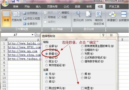
The next step is the third step. We need to select any blank cell, then right-click the mouse and select "Paste Special" in the pop-up menu. This step is very important, please pay attention to it.

Step 4: Select "Value" in the pop-up dialog box and click "OK";
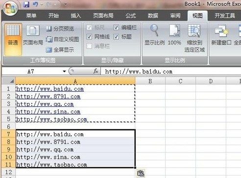
The fifth step is to delete the original cells with hyperlinks. If the amount of data is too large and deletion is too troublesome, you can create a new workbook and directly "Paste Special" the copied content. ” to a new workbook and then save it;
Method 2: Macro method
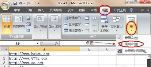
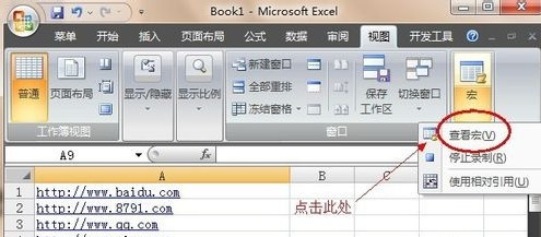
The first step is to open the "View" option, select "Macro", and select "Record Macro" in the drop-down box;
The second step is to enter the macro name;

The third step, click "Macro" - "View Macro" - select the corresponding macro - "Edit";

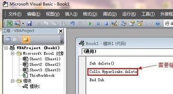
Step 4. In the pop-up macro editor, enter the corresponding code, specifically:
Sub ZapHyperlinks()
Cells.Hyperlinks.Delete
End Sub
Among them, the first and third lines are unchanged. Just change the content in the middle to "Cells.Hyperlinks.Delete" above, then close the editor;
Step 5: Click "Macro" - "View Macro" - "Execute" to complete the batch cancellation of hyperlinks;


How to delete hyperlinks in batches in Excel
The cells in a column in Excel all contain hyperlinks. You must manually delete hyperlinks one by one: right-click any cell in the column that contains a hyperlink and select "Cancel Hyperlink". Due to the huge number, only batch deletion method can be considered.
Open the Excel file, switch to the "View" tab, click "Macro" → "Record Macro", the "Record New Macro" window will appear, define a name in "Macro Name" as: RemoveHyperlinks, click "OK" quit;
Click "Macros" → "View Macros", select "RemoveHyperlinks" under "Macro Name" and click "Edit" to open the "Microsoft Visual Basic" editor and replace all the code in the right window with the following content , then save and close the VBA editor:
Sub RemoveHyperlinks()
'Remove all hyperlinks from the active sheet
ActiveSheet.Hyperlinks.Delete
End Sub
Click "Macros" → "View Macros", select "RemoveHyperlinks" under "Macro Name" and click "Execute" to remove the link to the worksheet.
The same purpose can be achieved with the following code:
Sub ZapHyperlinks()
Cells.Hyperlinks.Delete
End Sub
How to remove multiple hyperlinks in batches in Excel
Due to the huge number, only the batch deletion method can be considered.
1. Macro code removal method
Open the Excel file, switch to the "View" tab, click "Macro" → "Record Macro", the "Record New Macro" window will appear, define a name in "Macro Name" as: RemoveHyperlinks, click "OK" Exit; then click "Macros" → "View Macros", select "RemoveHyperlinks" under "Macro Name" and click "Edit" to open "Microsoft
Visual Basic" editor, replace all the code in the right window with the following content, then save and close the VBA editor:
Sub RemoveHyperlinks()
'Remove all hyperlinks from the active sheet
ActiveSheet.Hyperlinks.Delete
End Sub
Click "Macros" → "View Macros", select "RemoveHyperlinks" under "Macro Name" and click "Execute" to remove the link to the worksheet.
The same purpose can be achieved with the following code:
Sub ZapHyperlinks()
Cells.Hyperlinks.Delete
End Sub
2. Selective Paste Method
Right-click the column containing the hyperlink and select "Copy", then insert a blank column to the right of the column (left), then right-click the blank column and select "Paste Special",
In the "Paste Special" window that appears subsequently, click the "Value" option (careful people will find that when selecting options such as "Value", the "Paste Link" button becomes gray and unavailable. Naturally, the hyperlink will not be pasted), and finally keep the column, and then delete the column that originally contained the hyperlink.
3. The fastest way to delete hyperlinks in Excel
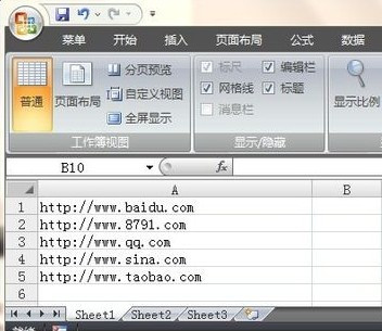
First select all cells with hyperlinks, copy them, and then press Enter, the hyperlinks will be gone!
The above is the detailed content of How to cancel a hyperlink in Excel at once. For more information, please follow other related articles on the PHP Chinese website!

Hot AI Tools

Undresser.AI Undress
AI-powered app for creating realistic nude photos

AI Clothes Remover
Online AI tool for removing clothes from photos.

Undress AI Tool
Undress images for free

Clothoff.io
AI clothes remover

Video Face Swap
Swap faces in any video effortlessly with our completely free AI face swap tool!

Hot Article
Hot Tools

Notepad++7.3.1
Easy-to-use and free code editor

SublimeText3 Chinese version
Chinese version, very easy to use

Zend Studio 13.0.1
Powerful PHP integrated development environment

Dreamweaver CS6
Visual web development tools

SublimeText3 Mac version
God-level code editing software (SublimeText3)
Hot Topics


 How to Create a Timeline Filter in Excel
Apr 03, 2025 am 03:51 AM
How to Create a Timeline Filter in Excel
Apr 03, 2025 am 03:51 AM
In Excel, using the timeline filter can display data by time period more efficiently, which is more convenient than using the filter button. The Timeline is a dynamic filtering option that allows you to quickly display data for a single date, month, quarter, or year. Step 1: Convert data to pivot table First, convert the original Excel data into a pivot table. Select any cell in the data table (formatted or not) and click PivotTable on the Insert tab of the ribbon. Related: How to Create Pivot Tables in Microsoft Excel Don't be intimidated by the pivot table! We will teach you basic skills that you can master in minutes. Related Articles In the dialog box, make sure the entire data range is selected (
 If You Don't Rename Tables in Excel, Today's the Day to Start
Apr 15, 2025 am 12:58 AM
If You Don't Rename Tables in Excel, Today's the Day to Start
Apr 15, 2025 am 12:58 AM
Quick link Why should tables be named in Excel How to name a table in Excel Excel table naming rules and techniques By default, tables in Excel are named Table1, Table2, Table3, and so on. However, you don't have to stick to these tags. In fact, it would be better if you don't! In this quick guide, I will explain why you should always rename tables in Excel and show you how to do this. Why should tables be named in Excel While it may take some time to develop the habit of naming tables in Excel (if you don't usually do this), the following reasons illustrate today
 You Need to Know What the Hash Sign Does in Excel Formulas
Apr 08, 2025 am 12:55 AM
You Need to Know What the Hash Sign Does in Excel Formulas
Apr 08, 2025 am 12:55 AM
Excel Overflow Range Operator (#) enables formulas to be automatically adjusted to accommodate changes in overflow range size. This feature is only available for Microsoft 365 Excel for Windows or Mac. Common functions such as UNIQUE, COUNTIF, and SORTBY can be used in conjunction with overflow range operators to generate dynamic sortable lists. The pound sign (#) in the Excel formula is also called the overflow range operator, which instructs the program to consider all results in the overflow range. Therefore, even if the overflow range increases or decreases, the formula containing # will automatically reflect this change. How to list and sort unique values in Microsoft Excel
 How to Format a Spilled Array in Excel
Apr 10, 2025 pm 12:01 PM
How to Format a Spilled Array in Excel
Apr 10, 2025 pm 12:01 PM
Use formula conditional formatting to handle overflow arrays in Excel Direct formatting of overflow arrays in Excel can cause problems, especially when the data shape or size changes. Formula-based conditional formatting rules allow automatic formatting to be adjusted when data parameters change. Adding a dollar sign ($) before a column reference applies a rule to all rows in the data. In Excel, you can apply direct formatting to the values or background of a cell to make the spreadsheet easier to read. However, when an Excel formula returns a set of values (called overflow arrays), applying direct formatting will cause problems if the size or shape of the data changes. Suppose you have this spreadsheet with overflow results from the PIVOTBY formula,

 How to change Excel table styles and remove table formatting
Apr 19, 2025 am 11:45 AM
How to change Excel table styles and remove table formatting
Apr 19, 2025 am 11:45 AM
This tutorial shows you how to quickly apply, modify, and remove Excel table styles while preserving all table functionalities. Want to make your Excel tables look exactly how you want? Read on! After creating an Excel table, the first step is usual
 Excel MATCH function with formula examples
Apr 15, 2025 am 11:21 AM
Excel MATCH function with formula examples
Apr 15, 2025 am 11:21 AM
This tutorial explains how to use MATCH function in Excel with formula examples. It also shows how to improve your lookup formulas by a making dynamic formula with VLOOKUP and MATCH. In Microsoft Excel, there are many different lookup/ref
 How to Use Excel's AGGREGATE Function to Refine Calculations
Apr 12, 2025 am 12:54 AM
How to Use Excel's AGGREGATE Function to Refine Calculations
Apr 12, 2025 am 12:54 AM
Quick Links The AGGREGATE Syntax
