

Visualize O(n) using Python.

introduce
In the fields of computer science and programming, understanding the efficiency of algorithms is crucial as it helps create software that is both optimized and performs quickly. Time complexity is an important concept in this context because it measures how an algorithm's running time changes as the input size grows. The commonly used time complexity class O(n) represents a linear relationship between input size and execution time.
definition
Algorithmic complexity in computer science is the evaluation of the resources required, such as time and space utilization, based on the input size of an algorithm. Furthermore, it supports our understanding of how fast an algorithm performs when its input size is taken into account. The main notation used to describe algorithm complexity is Big O notation (O(n)).
grammar
for i in range(n):
   # do something
A `for` loop runs a specific set of instructions based on a range from 0 to `n-1`, and performs an operation or set of operations on each iteration. where 'n' represents the number of iterations.
Under O(n) time complexity, as the input size 'n' increases, the execution time increases proportionally. As 'n' increases, the number of iterations of the loop and the time required to complete the loop will increase proportionally. Linear time complexity exhibits a direct proportional relationship between input size and execution time.
Any task or sequence of tasks can be executed in a loop regardless of input size 'n'. The main aspect to note here is that the loop executes 'n' iterations, resulting in linear time complexity.
algorithm
Step 1: Initialize a variable sum to 0
Step 2: Iterate over each element in the provided list
Step 3: Merge the element into the current sum value.
Step 4: The sum should be returned after the loop ends.
Step 5: End
method
Method 1: Relationship between drawing time and input size
Method 2: The relationship between drawing operations and input scale
Method 1: Plot the relationship between time and input size
Example
import time
import matplotlib.pyplot as plt
def algo_time(n):
sum = 0
for i in range(n):
sum += i
return sum
input_sizes = []
execution_times = []
for i in range(1000, 11000, 1000):
start_time = time.time()
algo_time(i)
end_time = time.time()
input_sizes.append(i)
execution_times.append(end_time - start_time)
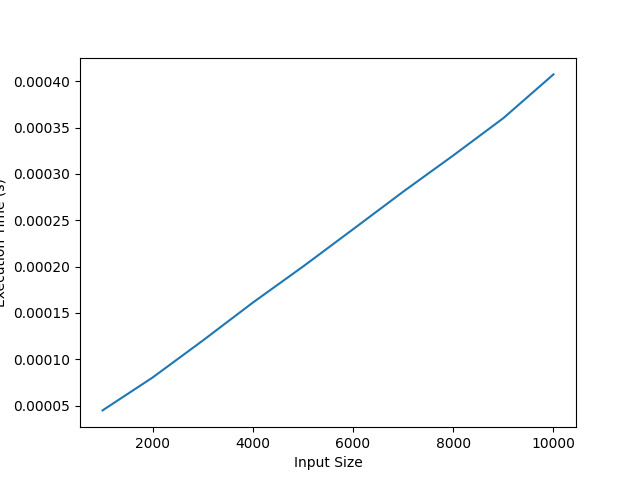
plt.plot(input_sizes, execution_times)
plt.xlabel('Input Size')
plt.ylabel('Execution Time (s)')
plt.show()
Output
This code is used to measure the running time of the `algo_time()` algorithm under different input sizes. We will store the input sizes we wish to test and their corresponding execution times in these lists.
Use a 'for' loop to iterate over a range of input sizes. In this case, the loop will run from 1000 until closer to 11000, incrementing by 1000 each time. To further illustrate, we plan to evaluate the algorithm by varying the value of 'n' from 1000 to 10000 in increments of 1000.
Inside the loop, we measure the execution time of the `algo_time()` function for each input size. To start tracking time, we use `time.time()` before calling the function, and stop it as soon as the function has finished running. We then store the duration in a variable called 'execution_time'.
We add each input value for a given input size ('n') and its corresponding execution time to their respective lists ('input_sizes' and 'execution_times').
After the loop completes, we have the data we need to generate the plot. 'plt.plot(input_sizes, execution_times)' generates a basic line chart using the data we collected. The x-axis shows 'input_sizes' values representing different input sizes.
'plt.xlabel()' and 'plt.ylabel()' are finally used to mark the meaning of the coordinate axes respectively, and calling the 'plt.show()' function enables us to present graphics.
By running this code, we can visualize the increase in execution time as the input size ('n') increases by plotting a graph. Assuming that the time complexity of the algorithm is O(n), we can approximate that there is an almost straight-line correlation between input size and execution time when plotting the graph.
Method 2: Relationship between drawing operation and input size
Example
import matplotlib.pyplot as plt

def algo_ops(n):
    ops = 0
    sum = 0
    for i in range(n):
        sum += i
        ops += 1
    ops += 1  # for the return statement
    return ops

input_sizes = []
operations = []

for i in range(1000, 11000, 1000):
    input_sizes.append(i)
    operations.append(algo_ops(i))

plt.plot(input_sizes, operations)
plt.xlabel

plt.xlabel('Input Size')
plt.ylabel('Number of Operations')
plt.show()
Output
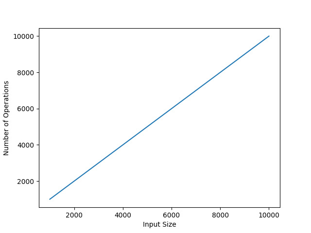
This code is designed to analyze the number of operations performed by the `algo_ops()` algorithm under different input sizes. By utilizing the `algo_ops()` function, you can calculate the sum of all values in the range from zero to the given input parameter 'n', while simultaneously tracking and recording every operation performed during each calculation.
We first import the 'matplotlib.pyplot' module, which allows us to create visualizations such as graphs.
Next, we define the algo_ops() function, which accepts an input number 'n'. Inside the function, we initialize two variables: 'ops' to count the number of operations, and 'sum' to store the cumulative sum of the numbers.
These arrays will store the dimensions we wish to examine and their corresponding execution durations.
One way we utilize iterative loops is to loop over multiple input scales. In this case, the loop execution range is from 1000 to 10000 (except 11000). This means we will evaluate the technique with variable 'n' between 1000 and 10000 in increments of 100.
In the loop, we calculate the performance of the `algo_time()` process for all input sizes. We use `time.time()` to start a stopwatch before calling the procedure, and end it directly after the subroutine has finished executing. Next, we save the time interval in a variable called 'execution_period'.
For each input size, we include the value of the input ('n') in a list called 'input_sizes'. Additionally, we append the corresponding processing times in the 'execution_times' collection.
After the loop is completed, we have accumulated the basic data needed to make the chart. The statement 'plt.plot(input_sizes, execution_times)' creates a basic line chart using the collected data. The values of 'input_sizes' are shown on the x-axis and represent different input sizes. The value of 'execution_times' is shown on the vertical axis and represents the time required to execute the `algo_time()` function with varying input sizes.
Finally, we label the coordinate system through 'plt.xlabel()' and 'plt.ylabel()' to show the meaning of each axis. Next, execute the 'plt.show()' function to render the graph.
Once we execute the program, the graph will show us how the processing time rises as the size of the input ('n') grows.
in conclusion
In conclusion, mastering time complexity and visualization in Python using Matplotlib is a valuable skill for any programmer seeking to create efficient and optimized software solutions. Understanding how algorithms behave at different input scales enables us to solve complex problems and build robust applications that deliver results in a timely and efficient manner.
The above is the detailed content of Visualize O(n) using Python.. For more information, please follow other related articles on the PHP Chinese website!

Hot AI Tools

Undresser.AI Undress
AI-powered app for creating realistic nude photos

AI Clothes Remover
Online AI tool for removing clothes from photos.

Undress AI Tool
Undress images for free

Clothoff.io
AI clothes remover

Video Face Swap
Swap faces in any video effortlessly with our completely free AI face swap tool!

Hot Article
Hot Tools

Notepad++7.3.1
Easy-to-use and free code editor

SublimeText3 Chinese version
Chinese version, very easy to use

Zend Studio 13.0.1
Powerful PHP integrated development environment

Dreamweaver CS6
Visual web development tools

SublimeText3 Mac version
God-level code editing software (SublimeText3)
Hot Topics


 How to solve the permissions problem encountered when viewing Python version in Linux terminal?
Apr 01, 2025 pm 05:09 PM
How to solve the permissions problem encountered when viewing Python version in Linux terminal?
Apr 01, 2025 pm 05:09 PM
Solution to permission issues when viewing Python version in Linux terminal When you try to view Python version in Linux terminal, enter python...
 How to avoid being detected by the browser when using Fiddler Everywhere for man-in-the-middle reading?
Apr 02, 2025 am 07:15 AM
How to avoid being detected by the browser when using Fiddler Everywhere for man-in-the-middle reading?
Apr 02, 2025 am 07:15 AM
How to avoid being detected when using FiddlerEverywhere for man-in-the-middle readings When you use FiddlerEverywhere...
 How to teach computer novice programming basics in project and problem-driven methods within 10 hours?
Apr 02, 2025 am 07:18 AM
How to teach computer novice programming basics in project and problem-driven methods within 10 hours?
Apr 02, 2025 am 07:18 AM
How to teach computer novice programming basics within 10 hours? If you only have 10 hours to teach computer novice some programming knowledge, what would you choose to teach...
 How to efficiently copy the entire column of one DataFrame into another DataFrame with different structures in Python?
Apr 01, 2025 pm 11:15 PM
How to efficiently copy the entire column of one DataFrame into another DataFrame with different structures in Python?
Apr 01, 2025 pm 11:15 PM
When using Python's pandas library, how to copy whole columns between two DataFrames with different structures is a common problem. Suppose we have two Dats...
 How does Uvicorn continuously listen for HTTP requests without serving_forever()?
Apr 01, 2025 pm 10:51 PM
How does Uvicorn continuously listen for HTTP requests without serving_forever()?
Apr 01, 2025 pm 10:51 PM
How does Uvicorn continuously listen for HTTP requests? Uvicorn is a lightweight web server based on ASGI. One of its core functions is to listen for HTTP requests and proceed...
 How to handle comma-separated list query parameters in FastAPI?
Apr 02, 2025 am 06:51 AM
How to handle comma-separated list query parameters in FastAPI?
Apr 02, 2025 am 06:51 AM
Fastapi ...
 How to solve permission issues when using python --version command in Linux terminal?
Apr 02, 2025 am 06:36 AM
How to solve permission issues when using python --version command in Linux terminal?
Apr 02, 2025 am 06:36 AM
Using python in Linux terminal...
 How to get news data bypassing Investing.com's anti-crawler mechanism?
Apr 02, 2025 am 07:03 AM
How to get news data bypassing Investing.com's anti-crawler mechanism?
Apr 02, 2025 am 07:03 AM
Understanding the anti-crawling strategy of Investing.com Many people often try to crawl news data from Investing.com (https://cn.investing.com/news/latest-news)...
