

How to measure the execution time efficiency of an algorithm?


On the basis of ignoring machine performance, we use algorithm time complexity to measure the execution time of the algorithm.
1. Time frequency
The time it takes to execute an algorithm cannot be calculated theoretically. It can only be known by running a test on the computer. But it is impossible and unnecessary for us to test every algorithm on the computer. We only need to know which algorithm takes more time and which algorithm takes less time. And The time an algorithm takes is proportional to the number of executions of statements in the algorithm. Which algorithm has more statements, the more time it takes. The number of statement executions in an algorithm is called statement frequency or time frequency. Denote it as T(n).
2. Time complexity
In the time frequency just mentioned, n is called the scale of the problem. When n keeps changing, the time frequency T(n) will also keep changing. But sometimes we want to know what pattern it shows when it changes. To this end, we introduce the concept of time complexity.
Generally, the number of times the basic operations in the algorithm are repeated is a function of the problem size n, represented by T(n). If there is an auxiliary function f(n), such that when n approaches At infinity, the limit value of T(n)/f(n) is a constant not equal to zero, then f(n) is said to be a function of the same order of magnitude as T(n). Denoted as T(n)=O(f(n)), O(f(n)) is called the asymptotic time complexity of the algorithm, or time complexity for short.
In various algorithms, if the number of statement executions in the algorithm is a constant, the time complexity is O(1). In addition, when the time frequency is different, the time complexity may be the same. For example, T(n)=n^2 3n 4 and T(n)=4n^2 2n 1 have different frequencies, but the time complexity is the same, both are O(n^2).
Arranged in increasing order of magnitude, common time complexity is:
Constant order O(1), logarithmic order O(log2n) (logarithm of n with base 2, the same below), linear order O( n),
Linear logarithmic order O(nlog2n), square order O(n^2), cubic order O(n^3),...,
kth power order O(n^k) , exponential order O(2^n). As the problem size n continues to increase, the above time complexity continues to increase, and the execution efficiency of the algorithm becomes lower.
Time performance analysis of the algorithm
(1) Time spent by the algorithm and statement frequency
The time spent by an algorithm = the sum of the execution time of each statement in the algorithm
The execution time of each statement = the number of executions of the statement (ie, frequency (Frequency Count)) × the time required to execute the statement once
After the algorithm is converted into a program, the time required to execute each statement depends on It depends on factors that are difficult to determine, such as the machine's instruction performance, speed, and the quality of the code generated by compilation.
To analyze the time consumption of an algorithm independently of the machine's software and hardware systems, assume that the time required to execute each statement once is unit time, and the time consumption of an algorithm is all the statements in the algorithm. The sum of frequencies.
To find the product C=A×B of two n-order square matrices, the algorithm is as follows:
  # define n 100 // n 可根据需要定义,这里假定为100
  void MatrixMultiply(int A[a],int B [n][n],int C[n][n])
  { //右边列为各语句的频度
  int i ,j ,k;
   for(i=0; i<n;j++) n+1
   for (j=0;j<n;j++) { n(n+1)
   C[i][j]=0; n
   for (k=0; k<n; k++) nn(n+1)
   C[i][j]=C[i][j]+A[i][k]*B[k][j];n
  }
}The sum of the frequencies of all statements in the algorithm (that is, the time of the algorithm Cost) is:
T(n)=nn(n 1) (1.1)
Analysis:
The loop control variable i of statement (1) should be increased to n , the test will not terminate until i=n is established. Therefore its frequency is n 1. But its loop body can only be executed n times. Statement (2), as a statement within the loop body of statement (1), should be executed n times, but statement (2) itself must be executed n 1 times, so the frequency of statement (2) is n(n 1). In the same way, the frequencies of sentences (3), (4) and (5) are n, nn(n 1) and n respectively.
The time consumption T(n) of the algorithm MatrixMultiply is a function of the matrix order n3.
(2) Problem scale and algorithm time complexity
The input amount of the algorithm to solve the problem is called the size of the problem (Size), which is generally represented by an integer.
The scale of the matrix product problem is the order of the matrix.
The size of a graph theory problem is the number of vertices or edges in the graph.
The time complexity (Time Complexity, also called time complexity) T(n) of an algorithm is the time consumption of the algorithm and is a function of the size n of the problem solved by the algorithm. When the size of the problem n approaches infinity, the order of magnitude (order) of the time complexity T(n) is called the asymptotic time complexity of the algorithm.
The time complexity T(n) of the algorithm MatrixMultidy is shown in equation (1.1). When n tends to infinity, there is obviously T(n)~O(n3);
This shows that , when n is large enough, the ratio of T(n) and n3 is a constant not equal to zero. That is, T(n) and n3 are of the same order, or T(n) and n3 are of the same order of magnitude. Denoted as T(n)=O(n3), it is the asymptotic time complexity of the algorithm MatrixMultiply.
(3) Asymptotic time complexity evaluation algorithm time performance
Mainly use the order of magnitude of algorithm time complexity (that is, the asymptotic time complexity of the algorithm) to evaluate the time performance of an algorithm.
The time complexity of the algorithm MatrixMultiply is generally T(n)=O(n3), and f(n)=n3 is the frequency of statement (5) in the algorithm. Next, we will give an example to illustrate how to find the time complexity of the algorithm.
Exchange the contents of i and j.
Temp=i;
i=j;
j=temp;
以上三条单个语句的频度均为1,该程序段的执行时间是一个与问题规模n无关的常数。算法的时间复杂度为常数阶,记作T(n)=O(1)。
注意:如果算法的执行时间不随着问题规模n的增加而增长,即使算法中有上千条语句,其执行时间也不过是一个较大的常数。此类算法的时间复杂度是O(1)。
变量计数之一:
   x=0;y=0;
   for(k-1;k<=n;k++)
   x++;
   for(i=1;i<=n;i++)
   for(j=1;j<=n;j++)
   y++;
一般情况下,对步进循环语句只需考虑循环体中语句的执行次数,忽略该语句中步长加1、终值判别、控制转移等成分。因此,以上程序段中频度最大的语句是(6),其频度为f(n)=n2,所以该程序段的时间复杂度为T(n)=O(n2)。
当有若干个循环语句时,算法的时间复杂度是由嵌套层数最多的循环语句中最内层语句的频度f(n)决定的。
变量计数之二:
x=1;
for(i=1;i<=n;i++)
for(j=1;j<=i;j++)
for(k=1;k<=j;k++)
x++;
该程序段中频度最大的语句是(5),内循环的执行次数虽然与问题规模n没有直接关系,但是却与外层循环的变量取值有关,而最外层循环的次数直接与n有关,因此可以从内层循环向外层分析语句(5)的执行次数:
则该程序段的时间复杂度为T(n)=O(n3/6+低次项)=O(n3)。
(4)算法的时间复杂度不仅仅依赖于问题的规模,还与输入实例的初始状态有关。
在数值A[0..n-1]中查找给定值K的算法大致如下:
i=n-1;
while(i>=0&&(A[i]!=k))
 i--;
return i;
此算法中的语句(3)的频度不仅与问题规模n有关,还与输入实例中A的各元素取值及K的取值有关:
①若A中没有与K相等的元素,则语句(3)的频度f(n)=n;
②若A的最后一个元素等于K,则语句(3)的频度f(n)是常数0。
The above is the detailed content of How to measure the execution time efficiency of an algorithm?. For more information, please follow other related articles on the PHP Chinese website!

Hot AI Tools

Undresser.AI Undress
AI-powered app for creating realistic nude photos

AI Clothes Remover
Online AI tool for removing clothes from photos.

Undress AI Tool
Undress images for free

Clothoff.io
AI clothes remover

Video Face Swap
Swap faces in any video effortlessly with our completely free AI face swap tool!

Hot Article
Hot Tools

Notepad++7.3.1
Easy-to-use and free code editor

SublimeText3 Chinese version
Chinese version, very easy to use

Zend Studio 13.0.1
Powerful PHP integrated development environment

Dreamweaver CS6
Visual web development tools

SublimeText3 Mac version
God-level code editing software (SublimeText3)
Hot Topics
 1671
1671
 14
1428
52
1329
25
1276
29
1256
24
14
1428
52
1329
25
1276
29
1256
24

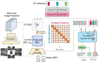 CLIP-BEVFormer: Explicitly supervise the BEVFormer structure to improve long-tail detection performance
Mar 26, 2024 pm 12:41 PM
CLIP-BEVFormer: Explicitly supervise the BEVFormer structure to improve long-tail detection performance
Mar 26, 2024 pm 12:41 PM
Written above & the author’s personal understanding: At present, in the entire autonomous driving system, the perception module plays a vital role. The autonomous vehicle driving on the road can only obtain accurate perception results through the perception module. The downstream regulation and control module in the autonomous driving system makes timely and correct judgments and behavioral decisions. Currently, cars with autonomous driving functions are usually equipped with a variety of data information sensors including surround-view camera sensors, lidar sensors, and millimeter-wave radar sensors to collect information in different modalities to achieve accurate perception tasks. The BEV perception algorithm based on pure vision is favored by the industry because of its low hardware cost and easy deployment, and its output results can be easily applied to various downstream tasks.
 Implementing Machine Learning Algorithms in C++: Common Challenges and Solutions
Jun 03, 2024 pm 01:25 PM
Implementing Machine Learning Algorithms in C++: Common Challenges and Solutions
Jun 03, 2024 pm 01:25 PM
Common challenges faced by machine learning algorithms in C++ include memory management, multi-threading, performance optimization, and maintainability. Solutions include using smart pointers, modern threading libraries, SIMD instructions and third-party libraries, as well as following coding style guidelines and using automation tools. Practical cases show how to use the Eigen library to implement linear regression algorithms, effectively manage memory and use high-performance matrix operations.
 Explore the underlying principles and algorithm selection of the C++sort function
Apr 02, 2024 pm 05:36 PM
Explore the underlying principles and algorithm selection of the C++sort function
Apr 02, 2024 pm 05:36 PM
The bottom layer of the C++sort function uses merge sort, its complexity is O(nlogn), and provides different sorting algorithm choices, including quick sort, heap sort and stable sort.
 Can artificial intelligence predict crime? Explore CrimeGPT's capabilities
Mar 22, 2024 pm 10:10 PM
Can artificial intelligence predict crime? Explore CrimeGPT's capabilities
Mar 22, 2024 pm 10:10 PM
The convergence of artificial intelligence (AI) and law enforcement opens up new possibilities for crime prevention and detection. The predictive capabilities of artificial intelligence are widely used in systems such as CrimeGPT (Crime Prediction Technology) to predict criminal activities. This article explores the potential of artificial intelligence in crime prediction, its current applications, the challenges it faces, and the possible ethical implications of the technology. Artificial Intelligence and Crime Prediction: The Basics CrimeGPT uses machine learning algorithms to analyze large data sets, identifying patterns that can predict where and when crimes are likely to occur. These data sets include historical crime statistics, demographic information, economic indicators, weather patterns, and more. By identifying trends that human analysts might miss, artificial intelligence can empower law enforcement agencies
 Improved detection algorithm: for target detection in high-resolution optical remote sensing images
Jun 06, 2024 pm 12:33 PM
Improved detection algorithm: for target detection in high-resolution optical remote sensing images
Jun 06, 2024 pm 12:33 PM
01 Outlook Summary Currently, it is difficult to achieve an appropriate balance between detection efficiency and detection results. We have developed an enhanced YOLOv5 algorithm for target detection in high-resolution optical remote sensing images, using multi-layer feature pyramids, multi-detection head strategies and hybrid attention modules to improve the effect of the target detection network in optical remote sensing images. According to the SIMD data set, the mAP of the new algorithm is 2.2% better than YOLOv5 and 8.48% better than YOLOX, achieving a better balance between detection results and speed. 02 Background & Motivation With the rapid development of remote sensing technology, high-resolution optical remote sensing images have been used to describe many objects on the earth’s surface, including aircraft, cars, buildings, etc. Object detection in the interpretation of remote sensing images
 Practice and reflections on Jiuzhang Yunji DataCanvas multi-modal large model platform
Oct 20, 2023 am 08:45 AM
Practice and reflections on Jiuzhang Yunji DataCanvas multi-modal large model platform
Oct 20, 2023 am 08:45 AM
1. The historical development of multi-modal large models. The photo above is the first artificial intelligence workshop held at Dartmouth College in the United States in 1956. This conference is also considered to have kicked off the development of artificial intelligence. Participants Mainly the pioneers of symbolic logic (except for the neurobiologist Peter Milner in the middle of the front row). However, this symbolic logic theory could not be realized for a long time, and even ushered in the first AI winter in the 1980s and 1990s. It was not until the recent implementation of large language models that we discovered that neural networks really carry this logical thinking. The work of neurobiologist Peter Milner inspired the subsequent development of artificial neural networks, and it was for this reason that he was invited to participate in this project.
 Application of algorithms in the construction of 58 portrait platform
May 09, 2024 am 09:01 AM
Application of algorithms in the construction of 58 portrait platform
May 09, 2024 am 09:01 AM
1. Background of the Construction of 58 Portraits Platform First of all, I would like to share with you the background of the construction of the 58 Portrait Platform. 1. The traditional thinking of the traditional profiling platform is no longer enough. Building a user profiling platform relies on data warehouse modeling capabilities to integrate data from multiple business lines to build accurate user portraits; it also requires data mining to understand user behavior, interests and needs, and provide algorithms. side capabilities; finally, it also needs to have data platform capabilities to efficiently store, query and share user profile data and provide profile services. The main difference between a self-built business profiling platform and a middle-office profiling platform is that the self-built profiling platform serves a single business line and can be customized on demand; the mid-office platform serves multiple business lines, has complex modeling, and provides more general capabilities. 2.58 User portraits of the background of Zhongtai portrait construction
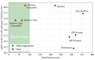 Add SOTA in real time and skyrocket! FastOcc: Faster inference and deployment-friendly Occ algorithm is here!
Mar 14, 2024 pm 11:50 PM
Add SOTA in real time and skyrocket! FastOcc: Faster inference and deployment-friendly Occ algorithm is here!
Mar 14, 2024 pm 11:50 PM
Written above & The author’s personal understanding is that in the autonomous driving system, the perception task is a crucial component of the entire autonomous driving system. The main goal of the perception task is to enable autonomous vehicles to understand and perceive surrounding environmental elements, such as vehicles driving on the road, pedestrians on the roadside, obstacles encountered during driving, traffic signs on the road, etc., thereby helping downstream modules Make correct and reasonable decisions and actions. A vehicle with self-driving capabilities is usually equipped with different types of information collection sensors, such as surround-view camera sensors, lidar sensors, millimeter-wave radar sensors, etc., to ensure that the self-driving vehicle can accurately perceive and understand surrounding environment elements. , enabling autonomous vehicles to make correct decisions during autonomous driving. Head