

The Beginner's Guide to Excel's Formulas and Functions

Excel Functions and Formulas: Getting Started Guide
Excel's functions and formulas are its core functions, both of which perform calculations, but are created, function and work in different ways. This article will explain both in an easy-to-understand manner to help you become an Excel expert. If you don't understand any terms, please refer to our Excel Glossary.
Detailed explanation of functions and formulas
The main difference between a formula and a function is that anyone can create a formula, and a function is predefined by a Microsoft programmer.
Excel formula
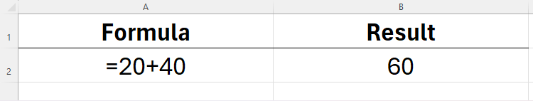
Excel formulas are used to perform basic mathematical calculations. Create a formula, first enter the equal sign (=), and then write the calculated parameters.
For example, enter:
in cell B2<code>=20+40</code>
Press Enter, Excel adds 20 and 40, and the result (60) will be displayed in the cell where the formula is entered.
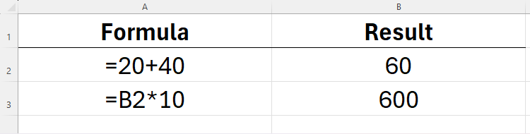
Excel can also calculate the values already in the spreadsheet. Enter:
in cell B3<code>=B2*10</code>
Press Enter to multiply the value in cell B2 by 10.
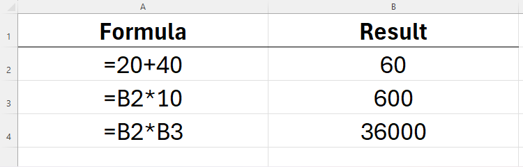
Same, enter:
in cell B4<code>=B2*B3</code>
Press Enter to multiply the values in cells B2 (60) and B3 (600) to a result of 36,000.
When creating an Excel formula, the number of parameters is not limited. For example, enter:
in cell B5<code>=B3*5-(2+8)</code>
Add 2 and 8, then multiply the value in B3 by 5, and subtract the former by the latter, and the result is 2,990.
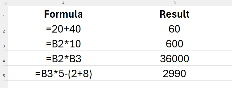
Excel follows the standard mathematical order of operations - PEMDAS (first brackets, then exponents, then multiplications and divisions, and finally adds and subtractions).
Excel function
Excel functions work similarly. They also start with an equal sign (=) and can perform calculations. However, Excel formulas are limited to basic mathematical operations, while functions are more powerful.
For example, the AVERAGE function can calculate the average value of a set of numbers, and the MAX function can find the maximum value in the range.
Excel functions follow a specific syntax:
<code>=a(b)</code>
where a is the function name (for example, AVERAGE or MAX), and b is the parameter used to enable the function to perform calculations.
For example, enter:
in cell A1<code>=AVERAGE(20,30)</code>
Press Enter to calculate the average of 20 and 30, and the result is 25.
We can also enter in cell B2:
<code>=AVERAGE(A1:A5)</code>
Let Excel calculate the average of all values in cells A1 to A5 (the colon indicates that the cells mentioned and all cells in between).
Excel has hundreds of functions, from the most basic functions to more complex functions. It's nearly impossible to remember all functions, especially considering that Microsoft developers are constantly adding new functions. Excel provides a function assistant to help you choose the most appropriate function and guide you through the entire process.
To start this assistant, click the "fx" icon above the first row of the spreadsheet, or press Shift F3.
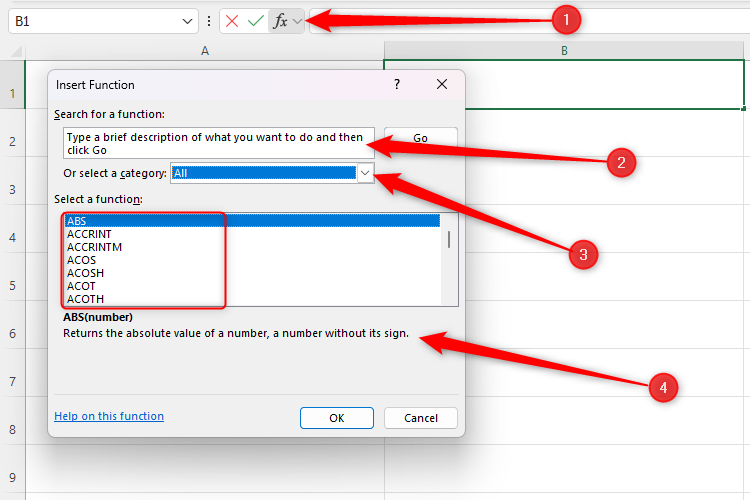
You can then enter some keywords in the Search Function field to find the function you want. The Select Category drop-down menu displays different groups of function, including financial, statistical, and logical categories. When you select a function in the list under category, you will see a short description of the function's function's function.
After finding the function you want to use, click OK. You will then see a new dialog box that guides you through the entire process.
Combination of formulas and functions
Formulas and functions can be used in combination. For example, enter:
<code>=20+40</code>
calculates the sum of the values in cells A1 to A10 and divides the sum by 2.
Cells and formula bars
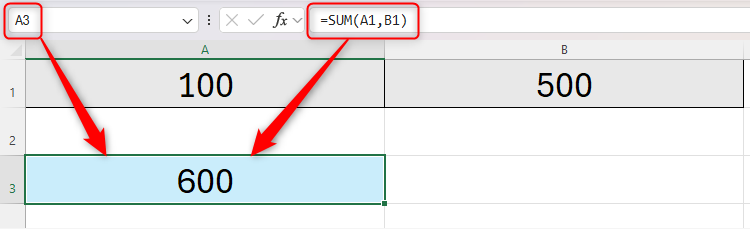
In Excel, once you enter a formula in a cell or use a function, the cell will display the calculation result instead of the formula itself. For example, when we enter:
in cell A3<code>=B2*10</code>
and press Enter, the calculation results will be displayed in cell A3, not the formula itself.
If you find an error that requires modification of the formula, you can use the formula bar located at the top of the Excel worksheet. You can also see the name box in the upper left corner, which indicates the active cell.
In other words, in the example below, the name box tells us that A3 is the active cell, the formula bar tells us what is entered in cell A3, and cell A3 itself shows the result of what we entered.
Copy formulas and functions
Excel provides convenient copying functions.
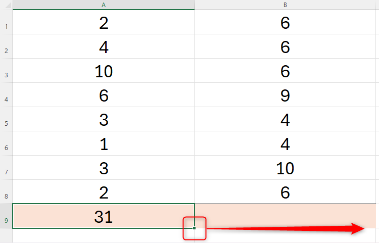
In the following example, we want to add all the values in cells A1 to A8, so we will enter:
in cell A9:<code>=B2*B3</code>
and press Enter.
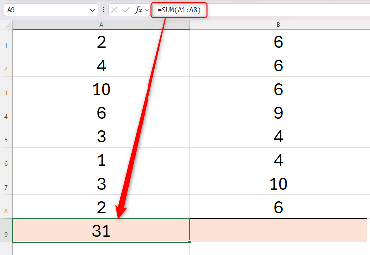
We also want to add the values in cells B1 to B8. However, instead of entering the new formula using the SUM function in B9, we can:
- Select cell A9, press Ctrl C, and then press Ctrl V in cell B9, or
- Drag the fill handle in the lower right corner of cell A9 to cell B9.
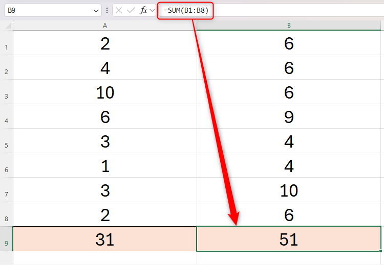
Because the cell references in the formula are relative by default, the method of calculating the values of cells A1 to A8 entered in cell A9 is also suitable for calculating the values of cells B1 to B8 in B9.
In some cases, you may not want the references in the formula to be relative. In this case, take some time to understand the difference between relative citations, absolute citations and mixed citations.
10 commonly used basic functions
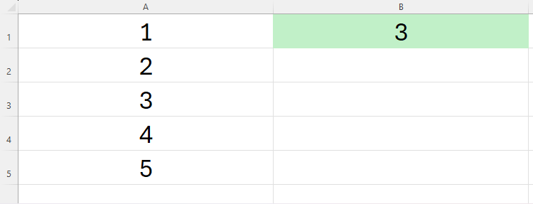
If you are new to Excel or its functions, open a new spreadsheet and enter some random values in cells A1 to A9 (A10 is left blank). Then, try some of the following functions:
| 在单元格 | 输入以下内容并按 Enter 键 | 功能 |
|---|---|---|
| B1 | =SUM(A1:A10) | SUM 函数将 A1 到 A10 单元格中的所有值相加。 |
| B2 | =AVERAGE(A1:A10) | AVERAGE 函数将计算 A1 到 A10 单元格中所有值的平均值。 |
| B3 | =CONCAT(A1:A3) | CONCAT 函数将 A1 到 A3 单元格中的所有值连接在一起。 |
| B4 | =COUNT(A1:A10) | COUNT 函数将告诉您 A1 到 A10 中包含数字的单元格数量。 |
| B5 | =COUNTA(A1:A10) | COUNTA 函数将告诉您包含任何值的单元格数量(换句话说,非空单元格)。 |
| B6 | =COUNTBLANK(A1:A10) | COUNTBLANK 函数将告诉您 A1 到 A10 中空白单元格的数量。 |
| B7 | =MIN(A1:A10) | 这将告诉您 A1 到 A10 单元格中最小的数字。 |
| B8 | =MAX(A1:A10) | 这将告诉您 A1 到 A10 单元格中最大的数字。 |
| B9 | =TODAY() | 易失性 TODAY 函数返回今天的日期。 |
| B10 | =RAND() | 易失性 RAND 函数返回 0 到 1 之间的随机数。 |
Volatile functions are recalculated when you make any changes to an Excel spreadsheet or reopen the spreadsheet.
5 more advanced functions
In a new worksheet or new workbook, enter Laura, Lucy, Liam, Lilly, Liz, and Luke in cells A1 to A6, and enter the numbers 1 to 6 in cells B1 to B6.
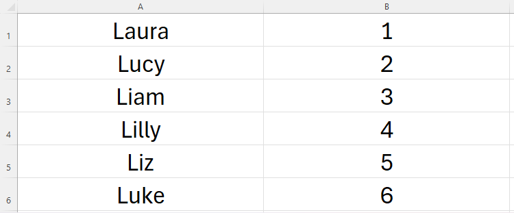
Now, try some of the following functions:
| 在单元格 | 输入以下内容并按 Enter 键 | 功能 |
|---|---|---|
| C1 | =IF(B6>1,"YES","NO") | IF 函数将评估单元格 B6 中的值是否大于 1,如果大于 1 则返回“YES”,否则返回“NO”。在本例中,它将返回“YES”。 |
| C2 | =VLOOKUP("Liam",A1:B6,2) | VLOOKUP 函数将在单元格 A1 到 B6 中查找“Liam”,返回在第二列中找到该单词的数字。在本例中,它将返回“3”。 |
| C3 | =SUMIF(A1:B6,"Li*",B1:B6) | SUMIF 函数将在单元格 A1 到 B6 中查找以“Li”开头的值,返回在满足此条件的单元格 B1 到 B6 中的值的总和。在本例中,它将返回“12”,因为 Liam、Lilly 和 Liz 旁边的数字加起来是 12。 |
| C4 | =COUNTIF(B1:B6,3) | COUNTIF 函数将告诉您 B1 到 B6 中有多少个单元格包含数字 3。在本例中,它将返回“1”,因为只有单元格 B3 包含此值。 |
| C5 | =LEFT(A1,3) | LEFT 函数将告诉您单元格 A1 中最左边的三个字符,在本例中是“Lau”。 |
Learning Excel's formulas and functions is a continuous learning process! We also have a lot of articles about Excel to help you become an Excel power user.
The above is the detailed content of The Beginner's Guide to Excel's Formulas and Functions. For more information, please follow other related articles on the PHP Chinese website!

Hot AI Tools

Undresser.AI Undress
AI-powered app for creating realistic nude photos

AI Clothes Remover
Online AI tool for removing clothes from photos.

Undress AI Tool
Undress images for free

Clothoff.io
AI clothes remover

Video Face Swap
Swap faces in any video effortlessly with our completely free AI face swap tool!

Hot Article
Hot Tools

Notepad++7.3.1
Easy-to-use and free code editor

SublimeText3 Chinese version
Chinese version, very easy to use

Zend Studio 13.0.1
Powerful PHP integrated development environment

Dreamweaver CS6
Visual web development tools

SublimeText3 Mac version
God-level code editing software (SublimeText3)
Hot Topics


 How to Create a Timeline Filter in Excel
Apr 03, 2025 am 03:51 AM
How to Create a Timeline Filter in Excel
Apr 03, 2025 am 03:51 AM
In Excel, using the timeline filter can display data by time period more efficiently, which is more convenient than using the filter button. The Timeline is a dynamic filtering option that allows you to quickly display data for a single date, month, quarter, or year. Step 1: Convert data to pivot table First, convert the original Excel data into a pivot table. Select any cell in the data table (formatted or not) and click PivotTable on the Insert tab of the ribbon. Related: How to Create Pivot Tables in Microsoft Excel Don't be intimidated by the pivot table! We will teach you basic skills that you can master in minutes. Related Articles In the dialog box, make sure the entire data range is selected (
 If You Don't Rename Tables in Excel, Today's the Day to Start
Apr 15, 2025 am 12:58 AM
If You Don't Rename Tables in Excel, Today's the Day to Start
Apr 15, 2025 am 12:58 AM
Quick link Why should tables be named in Excel How to name a table in Excel Excel table naming rules and techniques By default, tables in Excel are named Table1, Table2, Table3, and so on. However, you don't have to stick to these tags. In fact, it would be better if you don't! In this quick guide, I will explain why you should always rename tables in Excel and show you how to do this. Why should tables be named in Excel While it may take some time to develop the habit of naming tables in Excel (if you don't usually do this), the following reasons illustrate today
 You Need to Know What the Hash Sign Does in Excel Formulas
Apr 08, 2025 am 12:55 AM
You Need to Know What the Hash Sign Does in Excel Formulas
Apr 08, 2025 am 12:55 AM
Excel Overflow Range Operator (#) enables formulas to be automatically adjusted to accommodate changes in overflow range size. This feature is only available for Microsoft 365 Excel for Windows or Mac. Common functions such as UNIQUE, COUNTIF, and SORTBY can be used in conjunction with overflow range operators to generate dynamic sortable lists. The pound sign (#) in the Excel formula is also called the overflow range operator, which instructs the program to consider all results in the overflow range. Therefore, even if the overflow range increases or decreases, the formula containing # will automatically reflect this change. How to list and sort unique values in Microsoft Excel
 How to Format a Spilled Array in Excel
Apr 10, 2025 pm 12:01 PM
How to Format a Spilled Array in Excel
Apr 10, 2025 pm 12:01 PM
Use formula conditional formatting to handle overflow arrays in Excel Direct formatting of overflow arrays in Excel can cause problems, especially when the data shape or size changes. Formula-based conditional formatting rules allow automatic formatting to be adjusted when data parameters change. Adding a dollar sign ($) before a column reference applies a rule to all rows in the data. In Excel, you can apply direct formatting to the values or background of a cell to make the spreadsheet easier to read. However, when an Excel formula returns a set of values (called overflow arrays), applying direct formatting will cause problems if the size or shape of the data changes. Suppose you have this spreadsheet with overflow results from the PIVOTBY formula,
 How to change Excel table styles and remove table formatting
Apr 19, 2025 am 11:45 AM
How to change Excel table styles and remove table formatting
Apr 19, 2025 am 11:45 AM
This tutorial shows you how to quickly apply, modify, and remove Excel table styles while preserving all table functionalities. Want to make your Excel tables look exactly how you want? Read on! After creating an Excel table, the first step is usual

 Excel MATCH function with formula examples
Apr 15, 2025 am 11:21 AM
Excel MATCH function with formula examples
Apr 15, 2025 am 11:21 AM
This tutorial explains how to use MATCH function in Excel with formula examples. It also shows how to improve your lookup formulas by a making dynamic formula with VLOOKUP and MATCH. In Microsoft Excel, there are many different lookup/ref
 How to Use Excel's AGGREGATE Function to Refine Calculations
Apr 12, 2025 am 12:54 AM
How to Use Excel's AGGREGATE Function to Refine Calculations
Apr 12, 2025 am 12:54 AM
Quick Links The AGGREGATE Syntax
