How to implement two-color characters in PPT_Operation tutorial to implement two-color characters in PPT

How to easily achieve the two-color effect of fonts in PPT documents? This problem often troubles many users. In order to solve this problem, PHP editor Xigua specially brings you a detailed operation tutorial. This tutorial will guide you step by step to master the production method of PPT two-color characters, allowing you to easily create visually stunning slides.

Open the PPT and type text in the text box. In the example, it is [I am Chinese]. You can adjust the size and font of the text as you like. Choose a color you like. The color chosen here is pink.

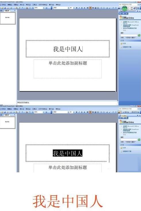
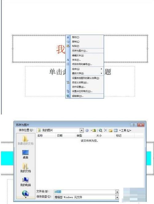
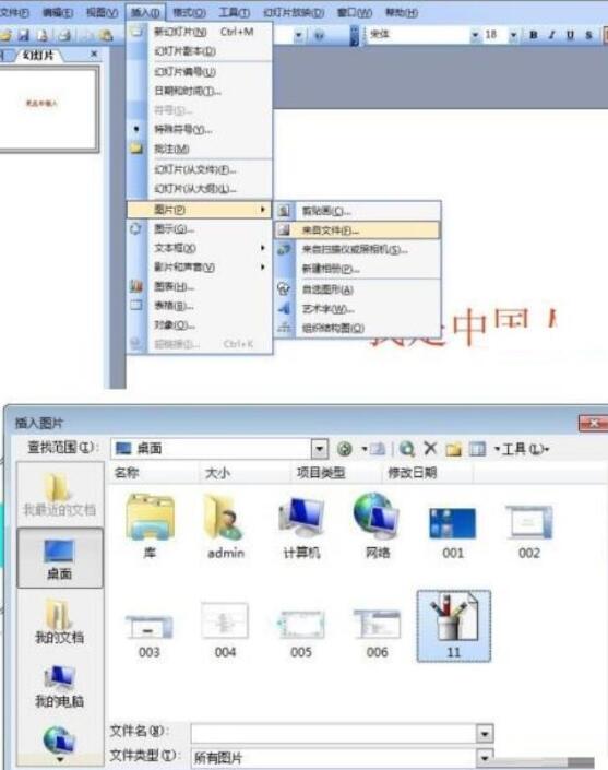
Right-click the mouse on the text box, select Save as picture, and select the image storage location in the dialog box. The desktop is selected here. In PPT, select Insert - Picture - From File - Find the picture you just saved. Change the color of the text in the original text box, here to blue.

Right-click the mouse on the inserted picture, select the Show Picture Tool, then click the crop icon, and pull down along the black border above the picture to about half of the word. Click the crop icon again.

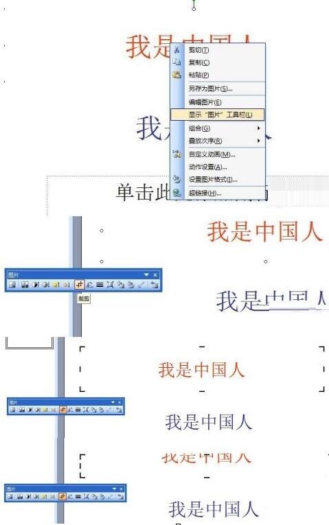
Select the cropped picture and use the arrow keys on the small keyboard to move the picture to cover the same part of the text in the text box. Press the ctrl key to select the picture and text box respectively for combination.

Play the slideshow and the final effect will appear.

The above is the detailed content of How to implement two-color characters in PPT_Operation tutorial to implement two-color characters in PPT. For more information, please follow other related articles on the PHP Chinese website!