

Detailed steps to find the square of a number in Excel table

php Xiaobian Youzi teaches you the detailed steps on how to find the square of a number in an Excel spreadsheet. First, select a cell and enter the value you want to square; then, use the multiplication operator () in the adjacent cell to multiply it by itself to get the square value. This simple operation can help you quickly calculate the square of any number and improve work efficiency.
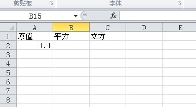
1. For example, ask for the square of cell A2 and put the obtained value in the position of cell B2.
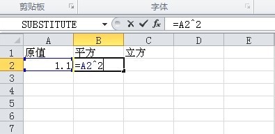
2. Just enter the formula in cell B2: =A2^2 and press Enter.
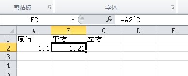
3. In this way, the square value of A2 is listed in cell B2.
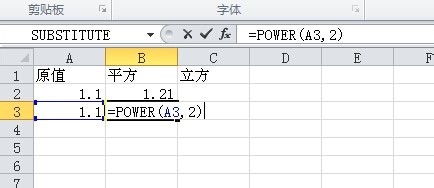
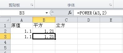
4. There is another way to find the square. For example, if you want the square of cell A3, just enter the formula in cell B3: =POWER(A3,2) and press Enter. .
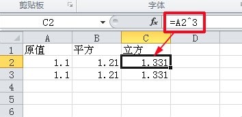
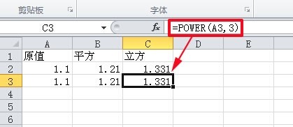
5. The following picture explains how to find a cube. Pay attention to the formula in the picture.
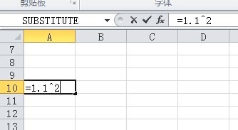
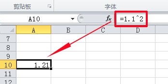
6. Excel can also directly find the square of a number. For example, if you want the square of 1.1, you can enter the formula in any cell, such as A10: =1.1^2 or =POWER(1.1,2) and press Enter.
The above is the detailed content of Detailed steps to find the square of a number in Excel table. For more information, please follow other related articles on the PHP Chinese website!

Hot AI Tools

Undresser.AI Undress
AI-powered app for creating realistic nude photos

AI Clothes Remover
Online AI tool for removing clothes from photos.

Undress AI Tool
Undress images for free

Clothoff.io
AI clothes remover

Video Face Swap
Swap faces in any video effortlessly with our completely free AI face swap tool!

Hot Article
Hot Tools

Notepad++7.3.1
Easy-to-use and free code editor

SublimeText3 Chinese version
Chinese version, very easy to use

Zend Studio 13.0.1
Powerful PHP integrated development environment

Dreamweaver CS6
Visual web development tools

SublimeText3 Mac version
God-level code editing software (SublimeText3)
Hot Topics
 1662
1662
 14
1419
52
1312
25
1262
29
1235
24
14
1419
52
1312
25
1262
29
1235
24

 If You Don't Rename Tables in Excel, Today's the Day to Start
Apr 15, 2025 am 12:58 AM
If You Don't Rename Tables in Excel, Today's the Day to Start
Apr 15, 2025 am 12:58 AM
Quick link Why should tables be named in Excel How to name a table in Excel Excel table naming rules and techniques By default, tables in Excel are named Table1, Table2, Table3, and so on. However, you don't have to stick to these tags. In fact, it would be better if you don't! In this quick guide, I will explain why you should always rename tables in Excel and show you how to do this. Why should tables be named in Excel While it may take some time to develop the habit of naming tables in Excel (if you don't usually do this), the following reasons illustrate today
 How to change Excel table styles and remove table formatting
Apr 19, 2025 am 11:45 AM
How to change Excel table styles and remove table formatting
Apr 19, 2025 am 11:45 AM
This tutorial shows you how to quickly apply, modify, and remove Excel table styles while preserving all table functionalities. Want to make your Excel tables look exactly how you want? Read on! After creating an Excel table, the first step is usual
 You Need to Know What the Hash Sign Does in Excel Formulas
Apr 08, 2025 am 12:55 AM
You Need to Know What the Hash Sign Does in Excel Formulas
Apr 08, 2025 am 12:55 AM
Excel Overflow Range Operator (#) enables formulas to be automatically adjusted to accommodate changes in overflow range size. This feature is only available for Microsoft 365 Excel for Windows or Mac. Common functions such as UNIQUE, COUNTIF, and SORTBY can be used in conjunction with overflow range operators to generate dynamic sortable lists. The pound sign (#) in the Excel formula is also called the overflow range operator, which instructs the program to consider all results in the overflow range. Therefore, even if the overflow range increases or decreases, the formula containing # will automatically reflect this change. How to list and sort unique values in Microsoft Excel
 How to Format a Spilled Array in Excel
Apr 10, 2025 pm 12:01 PM
How to Format a Spilled Array in Excel
Apr 10, 2025 pm 12:01 PM
Use formula conditional formatting to handle overflow arrays in Excel Direct formatting of overflow arrays in Excel can cause problems, especially when the data shape or size changes. Formula-based conditional formatting rules allow automatic formatting to be adjusted when data parameters change. Adding a dollar sign ($) before a column reference applies a rule to all rows in the data. In Excel, you can apply direct formatting to the values or background of a cell to make the spreadsheet easier to read. However, when an Excel formula returns a set of values (called overflow arrays), applying direct formatting will cause problems if the size or shape of the data changes. Suppose you have this spreadsheet with overflow results from the PIVOTBY formula,
 Excel MATCH function with formula examples
Apr 15, 2025 am 11:21 AM
Excel MATCH function with formula examples
Apr 15, 2025 am 11:21 AM
This tutorial explains how to use MATCH function in Excel with formula examples. It also shows how to improve your lookup formulas by a making dynamic formula with VLOOKUP and MATCH. In Microsoft Excel, there are many different lookup/ref

 Excel: Compare strings in two cells for matches (case-insensitive or exact)
Apr 16, 2025 am 11:26 AM
Excel: Compare strings in two cells for matches (case-insensitive or exact)
Apr 16, 2025 am 11:26 AM
The tutorial shows how to compare text strings in Excel for case-insensitive and exact match. You will learn a number of formulas to compare two cells by their values, string length, or the number of occurrences of a specific character, a
 How to Use Excel's AGGREGATE Function to Refine Calculations
Apr 12, 2025 am 12:54 AM
How to Use Excel's AGGREGATE Function to Refine Calculations
Apr 12, 2025 am 12:54 AM
Quick Links The AGGREGATE Syntax
