
 Software Tutorial
Office Software
How to draw a colorful and changeable heart-shaped pattern in Excel
Software Tutorial
Office Software
How to draw a colorful and changeable heart-shaped pattern in Excel
How to draw a colorful and changeable heart-shaped pattern in Excel

php editor Banana brings you the operation method of drawing a colorful and changeable heart shape chart in Excel. With simple steps, you can make beautiful heart-shaped patterns in Excel. Not only is this technique easy to learn, but it adds interest and visual appeal to your data charts. Let’s learn how to do this together!
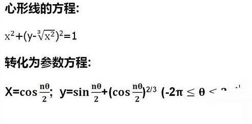
1. First, you need the heart-shaped function and parametric equation.
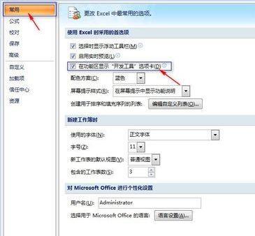
2. Click the win icon in the upper left corner of the menu bar and select [Excel Options] in the lower right corner.
3. In the pop-up [Excel Options] property box, select [Common], and under the [Preferences module when using Excel, select the [Show Development Tools tab in the ribbon] check box Check the box and click OK.
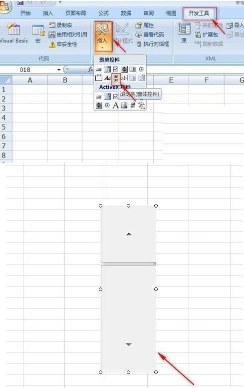
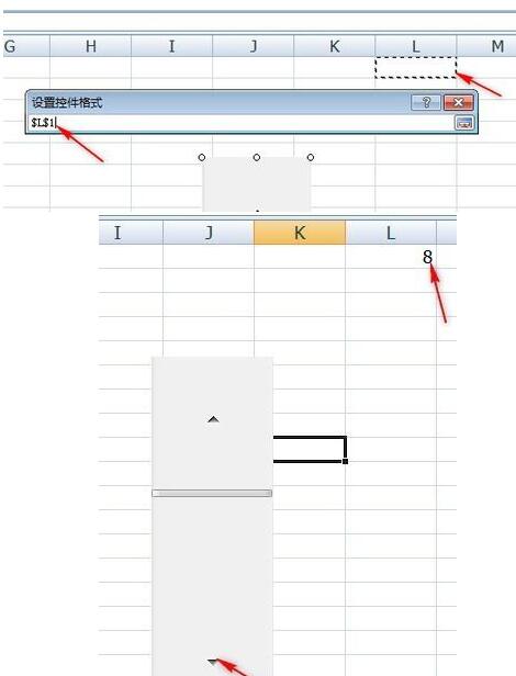
4. Click the [Development Tools] tab in the menu bar, click [Insert] in the [Controls] group, and then click [Scroll Bar] under [Form Control] 】. A cross mark will appear on the screen. Move the mouse to place the cross mark in the appropriate place. Click the left mouse button and a scroll bar will appear.
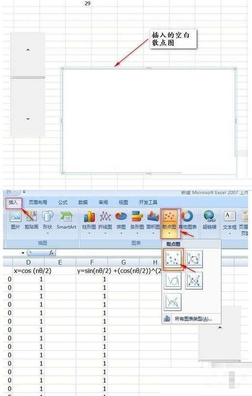
5. Now start setting the data. Divide the interval of θ into 200 equal parts, then calculate (nθ)/2, control the change of [n] through the [Scroll Bar], then calculate the values of x and y respectively through the parametric equation, and finally use the [Scatter Plot] 】Make corresponding graphics. The following steps are a bit complicated, so please read them carefully.
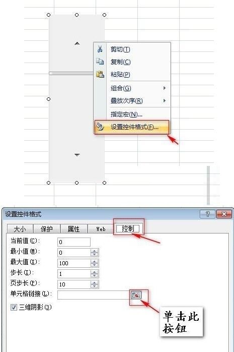
6. Select [Scroll Bar], right-click the mouse, and select [Format Control] in the pop-up menu. Then click [Control] in the Set Control Format Properties box, click the button to the right of [Cell Link], select the [L1] cell, press Enter to return, and then click [OK]. When we click the arrow of the [Scroll Bar], we will see that the number in the [L1] cell changes.
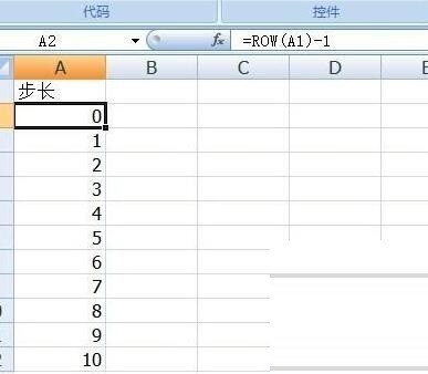
7. Enter [Step Size] in cell [A1], enter the formula [=ROW(A1)-1] in cell [A2], and select [A2] 】 cell, when the pointer turns into a black cross, drag down to 【A202】.
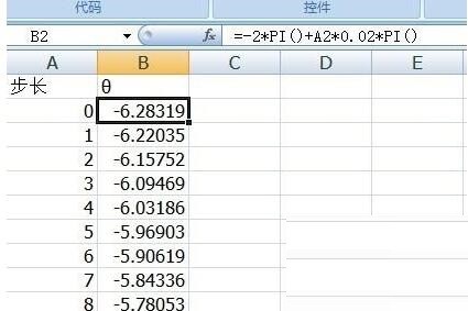
8. Enter [θ] in cell [B1], enter [=-2*PI() A2*0.02*PI()] in cell [B2], and select [ Cell B2], when the pointer turns into a black cross, drag down to [B202].
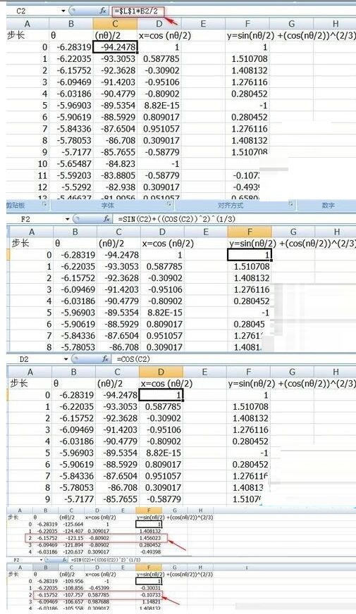
9. In [C1 [Cell Input] (nθ)/2 [,] C2 [Cell Input] = $K$1*B2/2 [, select [C2] Cell, when the pointer turns into a black cross, drag down to [C202].
In]D1[cell input]x=cos (nθ/2)[,]D2[cell input]=COS(C2)[, select the cell [D2], when the pointer turns black When the cross is on, drag down to [D202].
In】F1【Cell input】y=sin(nθ/2) (cos(nθ/2))^(2/3)【,】F2【Cell input】=SIN(C2) ((COS(C2))^2)^(1/3)【, select cell [F2], when the pointer turns into a black cross, drag down to [F202].
At this time, if we click on the arrow of the scroll bar, we will find that the data in columns C, D, and F will change as the value of n changes.
10. Select a blank cell, click Insert in the menu bar, click Scatter Plot in the chart area, select Scatter Plot with Data Markers Only [, get a blank scatter plot.
11. Select the blank scatter chart, right-click the mouse, and click [Select Data] in the pop-up dialog box, enter the Select Data Source Properties box, click [Add] —>] X-axis series value [selected area] = heart-shaped line $D$2:$D$202 [,] Y-axis series value [selected area] = heart-shaped line! $F$2:$F$202 [(The worksheet is called [Heart Shape Line]) Click twice in a row] OK [ to get the scatter plot sketch.
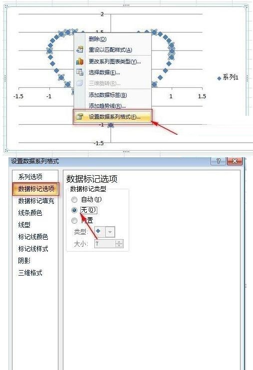
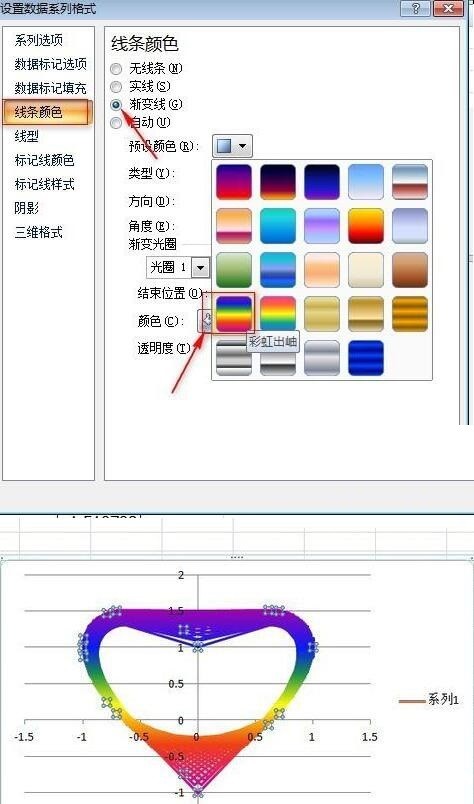
12. Select the heart-shaped trajectory in the chart, right-click, click] Set Data Series Format [—> click] Data Marker Options [, select] None [—> click] Line Color [, select 】Gradient color【Select【Rainbow Out of Pomelo】, click 】OK【.
The above is the detailed content of How to draw a colorful and changeable heart-shaped pattern in Excel. For more information, please follow other related articles on the PHP Chinese website!

Hot AI Tools

Undresser.AI Undress
AI-powered app for creating realistic nude photos

AI Clothes Remover
Online AI tool for removing clothes from photos.

Undress AI Tool
Undress images for free

Clothoff.io
AI clothes remover

Video Face Swap
Swap faces in any video effortlessly with our completely free AI face swap tool!

Hot Article
Hot Tools

Notepad++7.3.1
Easy-to-use and free code editor

SublimeText3 Chinese version
Chinese version, very easy to use

Zend Studio 13.0.1
Powerful PHP integrated development environment

Dreamweaver CS6
Visual web development tools

SublimeText3 Mac version
God-level code editing software (SublimeText3)
Hot Topics
 1658
1658
 14
1415
52
1309
25
1257
29
1231
24
14
1415
52
1309
25
1257
29
1231
24

 If You Don't Rename Tables in Excel, Today's the Day to Start
Apr 15, 2025 am 12:58 AM
If You Don't Rename Tables in Excel, Today's the Day to Start
Apr 15, 2025 am 12:58 AM
Quick link Why should tables be named in Excel How to name a table in Excel Excel table naming rules and techniques By default, tables in Excel are named Table1, Table2, Table3, and so on. However, you don't have to stick to these tags. In fact, it would be better if you don't! In this quick guide, I will explain why you should always rename tables in Excel and show you how to do this. Why should tables be named in Excel While it may take some time to develop the habit of naming tables in Excel (if you don't usually do this), the following reasons illustrate today
 You Need to Know What the Hash Sign Does in Excel Formulas
Apr 08, 2025 am 12:55 AM
You Need to Know What the Hash Sign Does in Excel Formulas
Apr 08, 2025 am 12:55 AM
Excel Overflow Range Operator (#) enables formulas to be automatically adjusted to accommodate changes in overflow range size. This feature is only available for Microsoft 365 Excel for Windows or Mac. Common functions such as UNIQUE, COUNTIF, and SORTBY can be used in conjunction with overflow range operators to generate dynamic sortable lists. The pound sign (#) in the Excel formula is also called the overflow range operator, which instructs the program to consider all results in the overflow range. Therefore, even if the overflow range increases or decreases, the formula containing # will automatically reflect this change. How to list and sort unique values in Microsoft Excel
 How to Format a Spilled Array in Excel
Apr 10, 2025 pm 12:01 PM
How to Format a Spilled Array in Excel
Apr 10, 2025 pm 12:01 PM
Use formula conditional formatting to handle overflow arrays in Excel Direct formatting of overflow arrays in Excel can cause problems, especially when the data shape or size changes. Formula-based conditional formatting rules allow automatic formatting to be adjusted when data parameters change. Adding a dollar sign ($) before a column reference applies a rule to all rows in the data. In Excel, you can apply direct formatting to the values or background of a cell to make the spreadsheet easier to read. However, when an Excel formula returns a set of values (called overflow arrays), applying direct formatting will cause problems if the size or shape of the data changes. Suppose you have this spreadsheet with overflow results from the PIVOTBY formula,
 How to change Excel table styles and remove table formatting
Apr 19, 2025 am 11:45 AM
How to change Excel table styles and remove table formatting
Apr 19, 2025 am 11:45 AM
This tutorial shows you how to quickly apply, modify, and remove Excel table styles while preserving all table functionalities. Want to make your Excel tables look exactly how you want? Read on! After creating an Excel table, the first step is usual
 Excel MATCH function with formula examples
Apr 15, 2025 am 11:21 AM
Excel MATCH function with formula examples
Apr 15, 2025 am 11:21 AM
This tutorial explains how to use MATCH function in Excel with formula examples. It also shows how to improve your lookup formulas by a making dynamic formula with VLOOKUP and MATCH. In Microsoft Excel, there are many different lookup/ref

 How to Use Excel's AGGREGATE Function to Refine Calculations
Apr 12, 2025 am 12:54 AM
How to Use Excel's AGGREGATE Function to Refine Calculations
Apr 12, 2025 am 12:54 AM
Quick Links The AGGREGATE Syntax
 Excel: Compare strings in two cells for matches (case-insensitive or exact)
Apr 16, 2025 am 11:26 AM
Excel: Compare strings in two cells for matches (case-insensitive or exact)
Apr 16, 2025 am 11:26 AM
The tutorial shows how to compare text strings in Excel for case-insensitive and exact match. You will learn a number of formulas to compare two cells by their values, string length, or the number of occurrences of a specific character, a
