

5 practical Excel tips to easily improve office efficiency!

In daily office work, Excel, as a commonly used office software, can help us process data, create tables and other tasks. This article introduces you to 5 practical Excel tips. Through these tips, you can easily improve office efficiency. There is no need for complicated operations, just master these tips and you will be able to use Excel more easily. Let’s take a look at these tips!
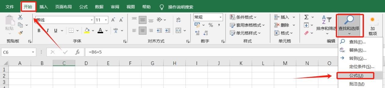
Tip 1: Quickly locate cells with formulas set
Function formulas are often used in Excel. Use the following method to quickly find the cells with formulas set.
Click [Start] → [Find and Select] → [Formula] in the Excel menu option list, and the cursor will automatically locate the cell where the function formula is set.
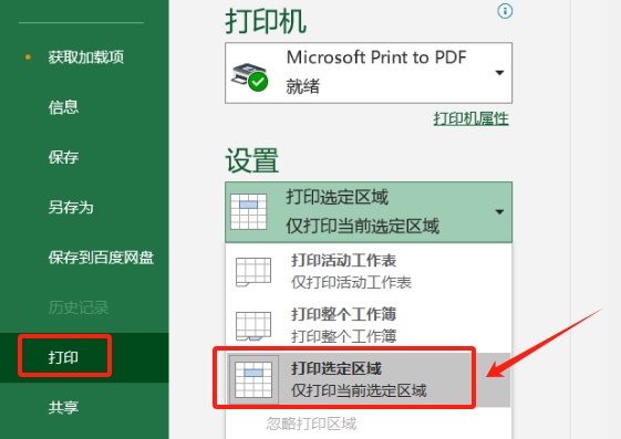
Tip 2: Print the selected area
To print an Excel table and only want to print the selected area, you can do it as follows.
First select the area that needs to be printed with the mouse, then click the menu tab [File], then click [Print] → [Settings] → [Print Selected Area], and finally click Print.
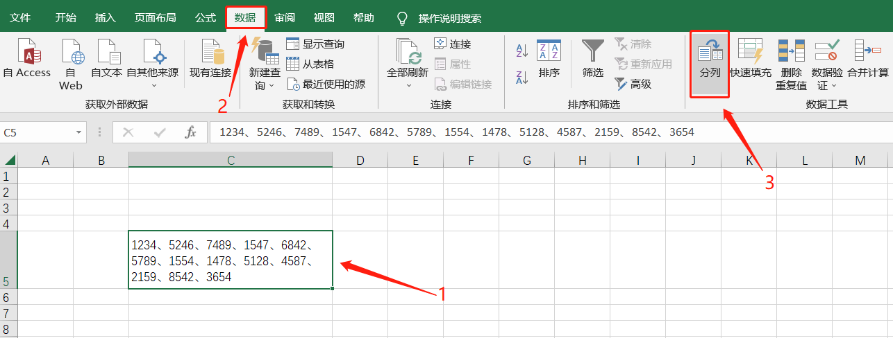
Tip 3: Split the data
If you have multiple data that need to be filled in Excel cells one by one, you can save a lot of time by using Excel's data splitting function.
First, select the cells where the data needs to be split, and then click the [Column] option in the menu tab [Data];
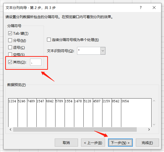
After the dialog box pops up, select [Delimiter], and then click [Next];
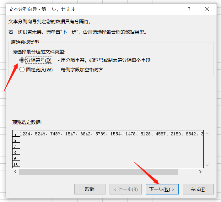
After the step 2 dialog box pops up, check the "Other" option and fill in the delimiter in the right box. For example, if the delimiter for data is a comma, fill in a comma, and if it is a period, fill in a comma, and then Click "Next";
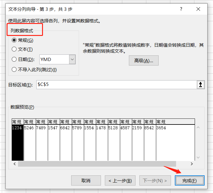
In step 3, click [General] under [Column Data Format], check the "Data Preview" and then click [Finish] to split the data into columns.
Tip 4: Prevent copying tables
If you don’t want to copy the completed form at will, you can do it as follows.
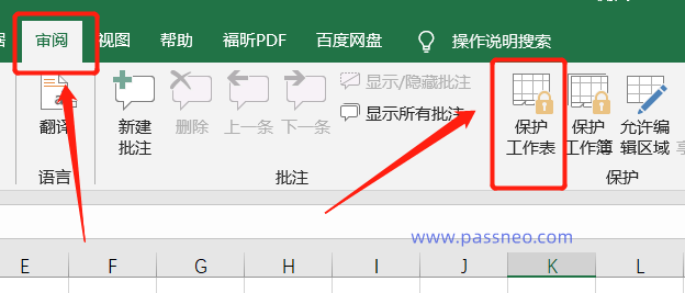
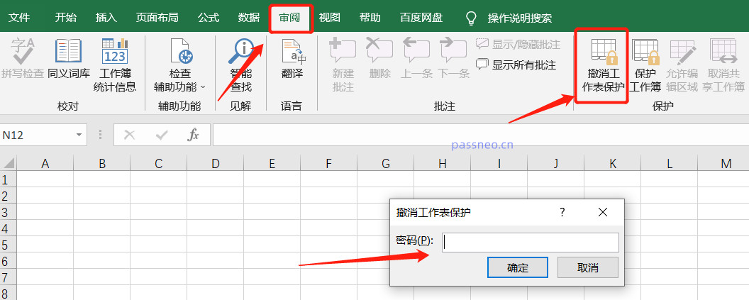
First, click [Review] → [Protect Worksheet] on the menu tab;
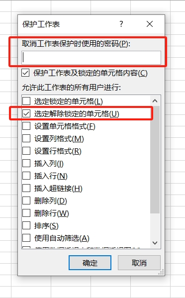
After the dialog box pops up, remove the checkmarks in front of [Select locked cells] and [Option to unlock locked cells], and enter the settings you want in the [Password to be used when unprotecting the worksheet] column. Password, finally click [OK] and re-enter the password once, and it is set.
After setting, the Excel table cannot be copied, but it cannot be edited or changed at the same time.
If you want to lift this restriction, click [Revoke Worksheet Protection] in the [Review] list of the menu tab. After the dialog box pops up, enter the originally set password to lift the restriction, and you can copy or Editor changed.
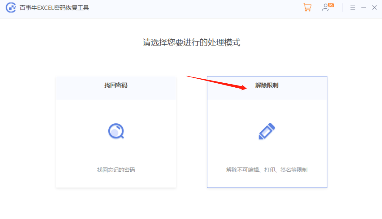
Because a password is required to remove restrictions, remember to remember it or save it. What to do if you accidentally forget it? In this case, it is best to use other tools, such as the Pepsi Niu Excel Password Recovery Tool, which can directly remove the "restrictions" of the Excel table without a password.
Click the [Unrestriction] module in the tool, and then import the Excel table.
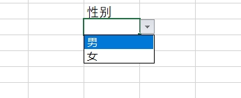
Tip 5: Set up Excel drop-down table
If there are certain cells in Excel that require repeated input, you can set them into drop-down tables to improve efficiency and make errors less likely.
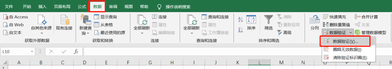
For example, if you need to enter the content of "male or female" in the table, select all the cells that need to enter the content, and then click [Data Validation] in the menu tab [Data] list; (Some Excel versions are "Data Validity")
After the dialog box pops up, select [Sequence] in the [Allow] list, enter "Male, Female" in the [Source] column (separate with English commas), and then click [OK] to set it up.
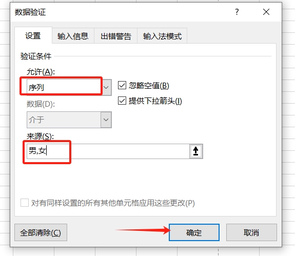
After setting, the selected cells can be filled in directly through the following list.
The above is the detailed content of 5 practical Excel tips to easily improve office efficiency!. For more information, please follow other related articles on the PHP Chinese website!

Hot AI Tools

Undresser.AI Undress
AI-powered app for creating realistic nude photos

AI Clothes Remover
Online AI tool for removing clothes from photos.

Undress AI Tool
Undress images for free

Clothoff.io
AI clothes remover

Video Face Swap
Swap faces in any video effortlessly with our completely free AI face swap tool!

Hot Article
Hot Tools

Notepad++7.3.1
Easy-to-use and free code editor

SublimeText3 Chinese version
Chinese version, very easy to use

Zend Studio 13.0.1
Powerful PHP integrated development environment

Dreamweaver CS6
Visual web development tools

SublimeText3 Mac version
God-level code editing software (SublimeText3)
Hot Topics
 1654
1654
 14
1413
52
1306
25
1252
29
1225
24
14
1413
52
1306
25
1252
29
1225
24

 If You Don't Rename Tables in Excel, Today's the Day to Start
Apr 15, 2025 am 12:58 AM
If You Don't Rename Tables in Excel, Today's the Day to Start
Apr 15, 2025 am 12:58 AM
Quick link Why should tables be named in Excel How to name a table in Excel Excel table naming rules and techniques By default, tables in Excel are named Table1, Table2, Table3, and so on. However, you don't have to stick to these tags. In fact, it would be better if you don't! In this quick guide, I will explain why you should always rename tables in Excel and show you how to do this. Why should tables be named in Excel While it may take some time to develop the habit of naming tables in Excel (if you don't usually do this), the following reasons illustrate today
 You Need to Know What the Hash Sign Does in Excel Formulas
Apr 08, 2025 am 12:55 AM
You Need to Know What the Hash Sign Does in Excel Formulas
Apr 08, 2025 am 12:55 AM
Excel Overflow Range Operator (#) enables formulas to be automatically adjusted to accommodate changes in overflow range size. This feature is only available for Microsoft 365 Excel for Windows or Mac. Common functions such as UNIQUE, COUNTIF, and SORTBY can be used in conjunction with overflow range operators to generate dynamic sortable lists. The pound sign (#) in the Excel formula is also called the overflow range operator, which instructs the program to consider all results in the overflow range. Therefore, even if the overflow range increases or decreases, the formula containing # will automatically reflect this change. How to list and sort unique values in Microsoft Excel
 How to change Excel table styles and remove table formatting
Apr 19, 2025 am 11:45 AM
How to change Excel table styles and remove table formatting
Apr 19, 2025 am 11:45 AM
This tutorial shows you how to quickly apply, modify, and remove Excel table styles while preserving all table functionalities. Want to make your Excel tables look exactly how you want? Read on! After creating an Excel table, the first step is usual
 How to Format a Spilled Array in Excel
Apr 10, 2025 pm 12:01 PM
How to Format a Spilled Array in Excel
Apr 10, 2025 pm 12:01 PM
Use formula conditional formatting to handle overflow arrays in Excel Direct formatting of overflow arrays in Excel can cause problems, especially when the data shape or size changes. Formula-based conditional formatting rules allow automatic formatting to be adjusted when data parameters change. Adding a dollar sign ($) before a column reference applies a rule to all rows in the data. In Excel, you can apply direct formatting to the values or background of a cell to make the spreadsheet easier to read. However, when an Excel formula returns a set of values (called overflow arrays), applying direct formatting will cause problems if the size or shape of the data changes. Suppose you have this spreadsheet with overflow results from the PIVOTBY formula,

 Excel MATCH function with formula examples
Apr 15, 2025 am 11:21 AM
Excel MATCH function with formula examples
Apr 15, 2025 am 11:21 AM
This tutorial explains how to use MATCH function in Excel with formula examples. It also shows how to improve your lookup formulas by a making dynamic formula with VLOOKUP and MATCH. In Microsoft Excel, there are many different lookup/ref
 How to Use Excel's AGGREGATE Function to Refine Calculations
Apr 12, 2025 am 12:54 AM
How to Use Excel's AGGREGATE Function to Refine Calculations
Apr 12, 2025 am 12:54 AM
Quick Links The AGGREGATE Syntax
 Excel: Compare strings in two cells for matches (case-insensitive or exact)
Apr 16, 2025 am 11:26 AM
Excel: Compare strings in two cells for matches (case-insensitive or exact)
Apr 16, 2025 am 11:26 AM
The tutorial shows how to compare text strings in Excel for case-insensitive and exact match. You will learn a number of formulas to compare two cells by their values, string length, or the number of occurrences of a specific character, a
