

Tips on deleting blank rows in Excel cells

Several points to delete blank rows in excel cells: 1. Only delete those with multiple consecutive blank rows such as 3
The content generated by alt carriage return, in excel, the function expression is char(10)
acsii code is alt 10
therefore
Use substitution to solve your problem. Strictly follow what I tell you and don’t act arbitrarily
ctrl H
The content entered in the search content box is invisible characters, the method is
Press the alt key without letting go, then press 10
in the small numeric keyboard areaRelease alt, press and hold alt again, enter 10 in the small numeric keyboard area again, release alt, press alt again and hold, enter 10 in the small numeric keyboard area again
That is, you need to press alt three times in total and enter 10
The replacement content is also an invisible character, which is a secondary alt 10
Then click Replace All. A pop-up window will tell you how many times it has been replaced. Confirm this window, and then click Replace All. It will also tell you how many times it has been successful. Repeat this until it prompts that the content cannot be found, and your request is completed.
Key points, 1. Press alt when you should press it, and release it when you should release it.
2. The small numeric keyboard area refers to the right side of the keyboard, not the top
3. Only replace them all multiple times.
How to delete blank rows in Excel worksheet
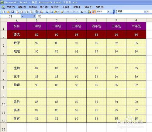
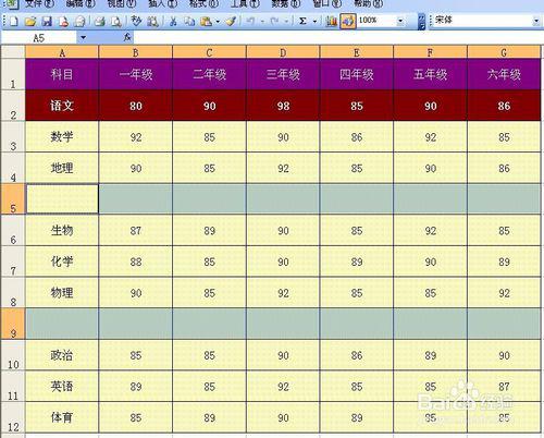
First we open the worksheet where we need to delete blank rows in batches. As shown in the figure, we can see that there are blank rows in this table.
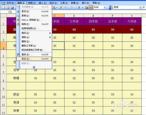
After opening, we move the mouse to the menu bar. There is an "Edit" button in the menu bar. Click the button, and in the drop-down option, we click the "Locate" button.
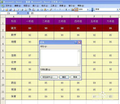
After clicking the "Position" button, the dialog box as shown in the figure will pop up. At this time, we click "Positioning Conditions".
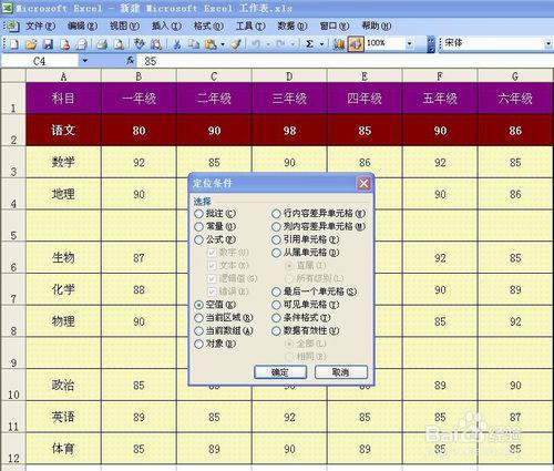
After clicking "Positioning Conditions", the following situation will appear. At this time, we select the "Null Value" button, and then click the "OK" button below.
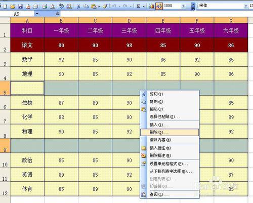
After clicking the "OK" button, the picture will appear. At this time, we can see that the blank rows have been selected. Then at this time, we can move the mouse to a blank row and click the right mouse button.
After clicking the right button of the mouse, a drop-down menu will appear. In the drop-down menu, we click the "Delete" button.
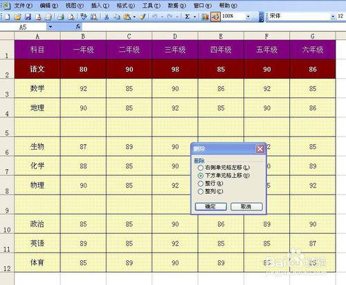
After clicking the "Delete" button, the dialog box as shown in the figure will pop up. At this time, we select "Move the lower cells up" and then click the "OK" button below.
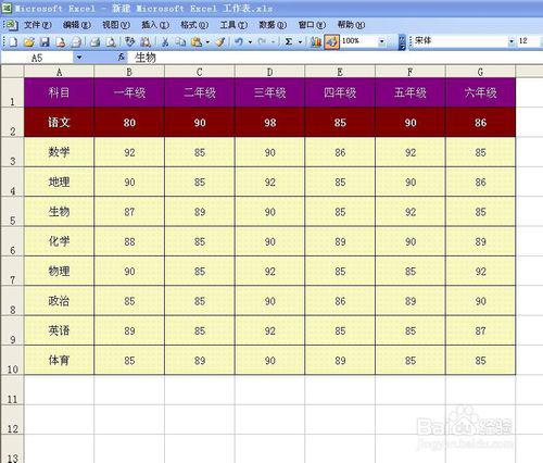
After clicking the "OK" button, the image shown in the figure will appear. At this time, we can see that the previously existing blank lines have been deleted by us in batches.
How to delete blank rows in excel
Method/Step
First we open the worksheet where we need to delete blank rows in batches. As shown in the figure, we can see that there are blank rows in this table.
After opening, we move the mouse to the menu bar. There is an "Edit" button in the menu bar. Click the button, and in the drop-down option, we click the "Locate" button.
After clicking the "Position" button, the dialog box as shown in the figure will pop up. At this time, we click "Positioning Conditions".
After clicking "Positioning Conditions", the following situation will appear. At this time, we select the "Null Value" button, and then click the "OK" button below.
After clicking the "OK" button, the picture will appear. At this time, we can see that the blank rows have been selected. Then at this time, we can move the mouse to a blank row and click the right mouse button.
After clicking the right button of the mouse, a drop-down menu will appear. In the drop-down menu, we click the "Delete" button.
After clicking the "Delete" button, the dialog box as shown in the figure will pop up. At this time, we select "Move the lower cells up" and then click the "OK" button below.
After clicking the "OK" button, the image shown in the figure will appear. At this time, we can see that the previously existing blank lines have been deleted by us in batches.
How to delete a blank row in excel
Delete blank lines directly
1
First open the excel table, place the mouse on the blank row, then right-click the mouse and select the "Delete" menu in the pop-up menu. (As shown below)
2
In the pop-up delete confirmation window, select delete the entire row, and then click the OK button. (As shown below)
3
Then repeat the above steps until all blank lines are deleted. (As shown below), this method is suitable for excel tables with relatively few blank lines.
END
Delete blank lines in batches
1
Open the excel table, then hold down the "Ctrl" key on the keyboard, and then use the mouse to continuously click on the blank rows to select all blank rows. (As shown below)
2
After selecting all the blank lines, right-click the mouse and select the delete function in the pop-up menu function. (As shown below)
3
Then in the confirmation window that pops up, select the entire row, and then click the OK button, so that all blank rows will be deleted. (As shown in Figure 1 and Figure 2 below)
END
Position and delete blank lines
The above two methods are still not fast enough. If there are many blank rows, you can locate the blank rows and first select all the data.
Among all the tools under the start menu, find the "Find and Select" tool in the upper right corner, click the drop-down icon, and select "Targeting Criteria".
In the positioning criteria window, select the null value, and then click the OK button.
After positioning the conditions, all empty values in the table have been selected, then right-click the mouse and select the delete menu.
5
In the delete confirmation window, select delete the entire row, and then click OK, so that all blank rows under the positioning are deleted successfully.
The above is the detailed content of Tips on deleting blank rows in Excel cells. For more information, please follow other related articles on the PHP Chinese website!

Hot AI Tools

Undresser.AI Undress
AI-powered app for creating realistic nude photos

AI Clothes Remover
Online AI tool for removing clothes from photos.

Undress AI Tool
Undress images for free

Clothoff.io
AI clothes remover

Video Face Swap
Swap faces in any video effortlessly with our completely free AI face swap tool!

Hot Article
Hot Tools

Notepad++7.3.1
Easy-to-use and free code editor

SublimeText3 Chinese version
Chinese version, very easy to use

Zend Studio 13.0.1
Powerful PHP integrated development environment

Dreamweaver CS6
Visual web development tools

SublimeText3 Mac version
God-level code editing software (SublimeText3)
Hot Topics
 1655
1655
 14
1413
52
1306
25
1252
29
1226
24
14
1413
52
1306
25
1252
29
1226
24

 If You Don't Rename Tables in Excel, Today's the Day to Start
Apr 15, 2025 am 12:58 AM
If You Don't Rename Tables in Excel, Today's the Day to Start
Apr 15, 2025 am 12:58 AM
Quick link Why should tables be named in Excel How to name a table in Excel Excel table naming rules and techniques By default, tables in Excel are named Table1, Table2, Table3, and so on. However, you don't have to stick to these tags. In fact, it would be better if you don't! In this quick guide, I will explain why you should always rename tables in Excel and show you how to do this. Why should tables be named in Excel While it may take some time to develop the habit of naming tables in Excel (if you don't usually do this), the following reasons illustrate today
 You Need to Know What the Hash Sign Does in Excel Formulas
Apr 08, 2025 am 12:55 AM
You Need to Know What the Hash Sign Does in Excel Formulas
Apr 08, 2025 am 12:55 AM
Excel Overflow Range Operator (#) enables formulas to be automatically adjusted to accommodate changes in overflow range size. This feature is only available for Microsoft 365 Excel for Windows or Mac. Common functions such as UNIQUE, COUNTIF, and SORTBY can be used in conjunction with overflow range operators to generate dynamic sortable lists. The pound sign (#) in the Excel formula is also called the overflow range operator, which instructs the program to consider all results in the overflow range. Therefore, even if the overflow range increases or decreases, the formula containing # will automatically reflect this change. How to list and sort unique values in Microsoft Excel
 How to change Excel table styles and remove table formatting
Apr 19, 2025 am 11:45 AM
How to change Excel table styles and remove table formatting
Apr 19, 2025 am 11:45 AM
This tutorial shows you how to quickly apply, modify, and remove Excel table styles while preserving all table functionalities. Want to make your Excel tables look exactly how you want? Read on! After creating an Excel table, the first step is usual
 How to Format a Spilled Array in Excel
Apr 10, 2025 pm 12:01 PM
How to Format a Spilled Array in Excel
Apr 10, 2025 pm 12:01 PM
Use formula conditional formatting to handle overflow arrays in Excel Direct formatting of overflow arrays in Excel can cause problems, especially when the data shape or size changes. Formula-based conditional formatting rules allow automatic formatting to be adjusted when data parameters change. Adding a dollar sign ($) before a column reference applies a rule to all rows in the data. In Excel, you can apply direct formatting to the values or background of a cell to make the spreadsheet easier to read. However, when an Excel formula returns a set of values (called overflow arrays), applying direct formatting will cause problems if the size or shape of the data changes. Suppose you have this spreadsheet with overflow results from the PIVOTBY formula,

 Excel MATCH function with formula examples
Apr 15, 2025 am 11:21 AM
Excel MATCH function with formula examples
Apr 15, 2025 am 11:21 AM
This tutorial explains how to use MATCH function in Excel with formula examples. It also shows how to improve your lookup formulas by a making dynamic formula with VLOOKUP and MATCH. In Microsoft Excel, there are many different lookup/ref
 How to Use Excel's AGGREGATE Function to Refine Calculations
Apr 12, 2025 am 12:54 AM
How to Use Excel's AGGREGATE Function to Refine Calculations
Apr 12, 2025 am 12:54 AM
Quick Links The AGGREGATE Syntax
 Excel: Compare strings in two cells for matches (case-insensitive or exact)
Apr 16, 2025 am 11:26 AM
Excel: Compare strings in two cells for matches (case-insensitive or exact)
Apr 16, 2025 am 11:26 AM
The tutorial shows how to compare text strings in Excel for case-insensitive and exact match. You will learn a number of formulas to compare two cells by their values, string length, or the number of occurrences of a specific character, a
