
 Software Tutorial
Office Software
Can a teacher of excel conditional statistical functions help me explain what the following functions mean? Thank you.
Software Tutorial
Office Software
Can a teacher of excel conditional statistical functions help me explain what the following functions mean? Thank you.
Can a teacher of excel conditional statistical functions help me explain what the following functions mean? Thank you.

Excel conditional statistical function teacher can help me explain what the following function means. Thank you
1. Two English double quotes "" represent blank characters;
Next, let’s introduce a very useful function-SUBSTITUTE(B2, ";", ""). This function can replace the English semicolon ";" in cell B2 with a null character to achieve the replacement effect. This function is very simple and easy to use, and is very useful when you need to replace specific characters. By using the SUBSTITUTE function, we can easily implement character replacement operations, making data processing more convenient and efficient.
3. SUBSTITUTE(SUBSTITUTE(B2,";",""),";","") is to replace the value of the result of SUBSTITUTE(B2,";","") again, and replace the Chinese points The sign ";" is also replaced.
4. LEN(B2) is to calculate the number of value characters in cell B2.
LEN(SUBSTITUTE(SUBSTITUTE(B2, ";", ""), ";", "")) function is used to calculate the number of characters after the semicolon is replaced in cell B2.
The subtraction of these two numbers is the number of Chinese and English semicolon ";" and ";" characters. Right now:
LEN(B2)-LEN(SUBSTITUTE(SUBSTITUTE(B2,";",""),";",""))
5. Finally execute the IF function. If the number of English semicolons LEN(B2)-LEN(SUBSTITUTE(SUBSTITUTE(B2,";",""),";","")) in B2 is not zero, then display the number LEN(B2 )-LEN(SUBSTITUTE(SUBSTITUTE(B2,";",""),";","")), otherwise "" will not be displayed. The formula is:
=IF(LEN(B2)-LEN(SUBSTITUTE(SUBSTITUTE(B2,";",""),";","")),LEN(B2)-LEN(SUBSTITUTE(SUBSTITUTE(B2," ;",""),";","")),"")
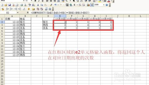
How to count functions based on multiple conditions in excel
Enter the function in cell e2 of the red box area, which will return the number of times this person appears on the corresponding date
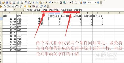
The multiplication of two equations means that two conditions are met at the same time. The function will count the number of true in an array composed of true and false, that is, the number of colleagues who meet the condition
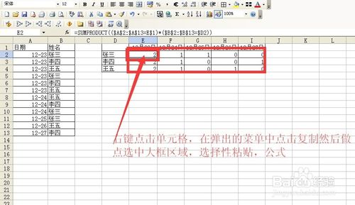
Right-click the cell, click Copy in the pop-up menu, then select the large box area, Paste Special, formula
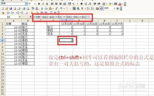
If you use the sum function, you can also achieve the same effect, but after completing the formula input, you need to press ctrl shift and press Enter to get the return value
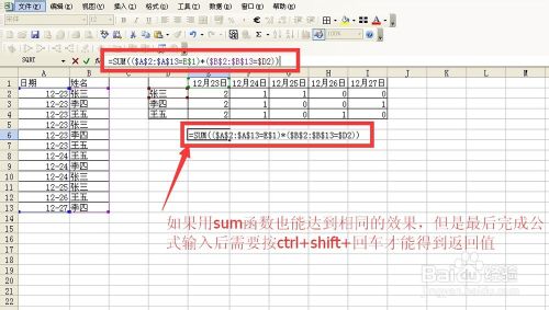
After pressing ctrl shift and pressing Enter, you can see that the formula in the edit bar has a pair of curly brackets, which is the symbol of the array formula
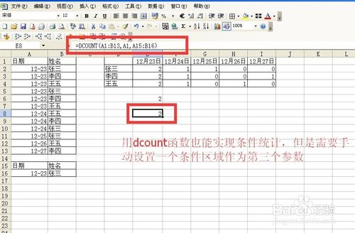
Conditional statistics can also be achieved using the dcount function, but you need to manually set a conditional area as the third parameter
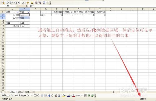
Or through automatic filtering, then select the data area in column b, then locate the visible cells, and observe the count in the lower right corner to get the same result
Note: When using dcount, the second parameter can specify the cell in the upper left corner of the condition area
The above is the detailed content of Can a teacher of excel conditional statistical functions help me explain what the following functions mean? Thank you.. For more information, please follow other related articles on the PHP Chinese website!

Hot AI Tools

Undresser.AI Undress
AI-powered app for creating realistic nude photos

AI Clothes Remover
Online AI tool for removing clothes from photos.

Undress AI Tool
Undress images for free

Clothoff.io
AI clothes remover

Video Face Swap
Swap faces in any video effortlessly with our completely free AI face swap tool!

Hot Article
Hot Tools

Notepad++7.3.1
Easy-to-use and free code editor

SublimeText3 Chinese version
Chinese version, very easy to use

Zend Studio 13.0.1
Powerful PHP integrated development environment

Dreamweaver CS6
Visual web development tools

SublimeText3 Mac version
God-level code editing software (SublimeText3)
Hot Topics
 1662
1662
 14
1418
52
1311
25
1261
29
1234
24
14
1418
52
1311
25
1261
29
1234
24

 If You Don't Rename Tables in Excel, Today's the Day to Start
Apr 15, 2025 am 12:58 AM
If You Don't Rename Tables in Excel, Today's the Day to Start
Apr 15, 2025 am 12:58 AM
Quick link Why should tables be named in Excel How to name a table in Excel Excel table naming rules and techniques By default, tables in Excel are named Table1, Table2, Table3, and so on. However, you don't have to stick to these tags. In fact, it would be better if you don't! In this quick guide, I will explain why you should always rename tables in Excel and show you how to do this. Why should tables be named in Excel While it may take some time to develop the habit of naming tables in Excel (if you don't usually do this), the following reasons illustrate today
 How to change Excel table styles and remove table formatting
Apr 19, 2025 am 11:45 AM
How to change Excel table styles and remove table formatting
Apr 19, 2025 am 11:45 AM
This tutorial shows you how to quickly apply, modify, and remove Excel table styles while preserving all table functionalities. Want to make your Excel tables look exactly how you want? Read on! After creating an Excel table, the first step is usual
 You Need to Know What the Hash Sign Does in Excel Formulas
Apr 08, 2025 am 12:55 AM
You Need to Know What the Hash Sign Does in Excel Formulas
Apr 08, 2025 am 12:55 AM
Excel Overflow Range Operator (#) enables formulas to be automatically adjusted to accommodate changes in overflow range size. This feature is only available for Microsoft 365 Excel for Windows or Mac. Common functions such as UNIQUE, COUNTIF, and SORTBY can be used in conjunction with overflow range operators to generate dynamic sortable lists. The pound sign (#) in the Excel formula is also called the overflow range operator, which instructs the program to consider all results in the overflow range. Therefore, even if the overflow range increases or decreases, the formula containing # will automatically reflect this change. How to list and sort unique values in Microsoft Excel
 How to Format a Spilled Array in Excel
Apr 10, 2025 pm 12:01 PM
How to Format a Spilled Array in Excel
Apr 10, 2025 pm 12:01 PM
Use formula conditional formatting to handle overflow arrays in Excel Direct formatting of overflow arrays in Excel can cause problems, especially when the data shape or size changes. Formula-based conditional formatting rules allow automatic formatting to be adjusted when data parameters change. Adding a dollar sign ($) before a column reference applies a rule to all rows in the data. In Excel, you can apply direct formatting to the values or background of a cell to make the spreadsheet easier to read. However, when an Excel formula returns a set of values (called overflow arrays), applying direct formatting will cause problems if the size or shape of the data changes. Suppose you have this spreadsheet with overflow results from the PIVOTBY formula,
 Excel MATCH function with formula examples
Apr 15, 2025 am 11:21 AM
Excel MATCH function with formula examples
Apr 15, 2025 am 11:21 AM
This tutorial explains how to use MATCH function in Excel with formula examples. It also shows how to improve your lookup formulas by a making dynamic formula with VLOOKUP and MATCH. In Microsoft Excel, there are many different lookup/ref

 How to Use Excel's AGGREGATE Function to Refine Calculations
Apr 12, 2025 am 12:54 AM
How to Use Excel's AGGREGATE Function to Refine Calculations
Apr 12, 2025 am 12:54 AM
Quick Links The AGGREGATE Syntax
 Excel: Compare strings in two cells for matches (case-insensitive or exact)
Apr 16, 2025 am 11:26 AM
Excel: Compare strings in two cells for matches (case-insensitive or exact)
Apr 16, 2025 am 11:26 AM
The tutorial shows how to compare text strings in Excel for case-insensitive and exact match. You will learn a number of formulas to compare two cells by their values, string length, or the number of occurrences of a specific character, a
