

How to calculate the average of a set of cells in Microsoft Excel

Suppose you have a set of numbers and you need to find their average. It could be anything, it could be the score on your student roster, it could be the number of visits to your website per month. It's completely impossible to manually calculate the average and populate it into an Excel column. If we have a perfect solution that automates the entire process, you don’t need to prioritize manual operations.
Keep reading to learn how to easily find the average of a group of cells in an Excel worksheet using a quick formula and populate the average of an entire column with a few simple clicks.
Solution
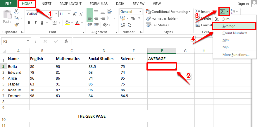
Step 1: Suppose you have a column named AVERAGE whose value needs to be calculated with each student Fill in the corresponding average of the values present in each row.
To do this, first click the first cell of the AVERAGE column .
Then make sure you are in the HOME tab at the top. Next, click the drop-down menu associated with the Sigma button and select Average from the list of options.
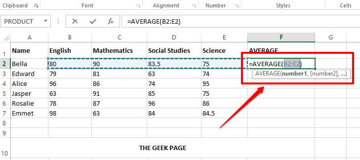
Step 2: All values appearing in the row of the selected cell will be automatically considered to calculate the average. In the example screenshot below, the average function auto-populates as =AVERAGE(B2:E2). Here B2:E2 represents all the cells from B2 to E2 in the Excel worksheet.
NOTE: If you need to make any changes, you can always edit the parameter list inside the AVERAGE() function. Suppose if you only need to find the average of cells C3 and D3, then your Average() function would be =AVERAGE(C3, D3). You can also provide static values as parameters in the Average() function. For example, your Average() function could also be =Average(4,87,34,1).
Step 3: Now if you press the Enter key, you can see that the average is calculated successfully. But the decimal point may not be present. If this is the case, right-click the cell and select "Format Cell " from the right-click context menu option.
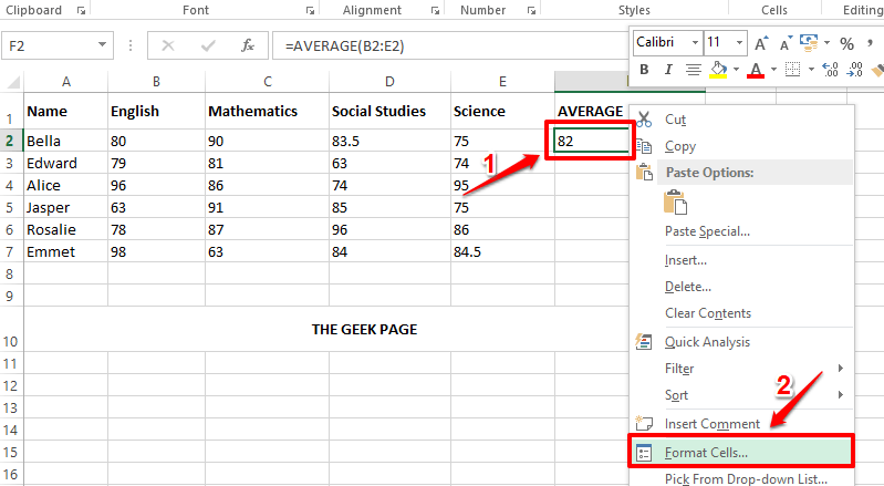
Step 4: In the Set CellsFormat window, make sure you are in step atab.
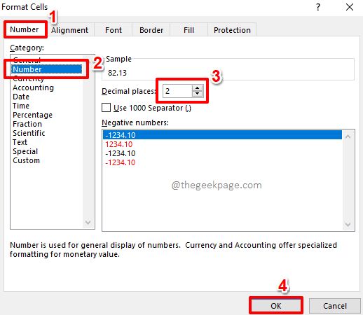
Now, under the Category option, click on Number.
To the right of , enter the number of decimal places you want in the decimal placesfiller. I gave 2 in the screenshot below.
Click the OK button after completion.
Step 5: You are here! Average values now also have decimal places visible. If you want to apply the same formula to the rest of the cells in the same column, just click and drag down the little square icon in the lower right corner of the formatted cell.
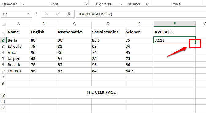
That’s it. Your formula to find the average of a group of cells is now successfully applied to all cells present in the same column.
The above is the detailed content of How to calculate the average of a set of cells in Microsoft Excel. For more information, please follow other related articles on the PHP Chinese website!

Hot AI Tools

Undresser.AI Undress
AI-powered app for creating realistic nude photos

AI Clothes Remover
Online AI tool for removing clothes from photos.

Undress AI Tool
Undress images for free

Clothoff.io
AI clothes remover

Video Face Swap
Swap faces in any video effortlessly with our completely free AI face swap tool!

Hot Article
Hot Tools

Notepad++7.3.1
Easy-to-use and free code editor

SublimeText3 Chinese version
Chinese version, very easy to use

Zend Studio 13.0.1
Powerful PHP integrated development environment

Dreamweaver CS6
Visual web development tools

SublimeText3 Mac version
God-level code editing software (SublimeText3)
Hot Topics


 Excel found a problem with one or more formula references: How to fix it
Apr 17, 2023 pm 06:58 PM
Excel found a problem with one or more formula references: How to fix it
Apr 17, 2023 pm 06:58 PM
Use an Error Checking Tool One of the quickest ways to find errors with your Excel spreadsheet is to use an error checking tool. If the tool finds any errors, you can correct them and try saving the file again. However, the tool may not find all types of errors. If the error checking tool doesn't find any errors or fixing them doesn't solve the problem, then you need to try one of the other fixes below. To use the error checking tool in Excel: select the Formulas tab. Click the Error Checking tool. When an error is found, information about the cause of the error will appear in the tool. If it's not needed, fix the error or delete the formula causing the problem. In the Error Checking Tool, click Next to view the next error and repeat the process. When not
 How to set the print area in Google Sheets?
May 08, 2023 pm 01:28 PM
How to set the print area in Google Sheets?
May 08, 2023 pm 01:28 PM
How to Set GoogleSheets Print Area in Print Preview Google Sheets allows you to print spreadsheets with three different print areas. You can choose to print the entire spreadsheet, including each individual worksheet you create. Alternatively, you can choose to print a single worksheet. Finally, you can only print a portion of the cells you select. This is the smallest print area you can create since you could theoretically select individual cells for printing. The easiest way to set it up is to use the built-in Google Sheets print preview menu. You can view this content using Google Sheets in a web browser on your PC, Mac, or Chromebook. To set up Google
 5 Tips to Fix Stdole32.tlb Excel Error in Windows 11
May 09, 2023 pm 01:37 PM
5 Tips to Fix Stdole32.tlb Excel Error in Windows 11
May 09, 2023 pm 01:37 PM
When you start Microsoft Word or Microsoft Excel, Windows very tediously tries to set up Office 365. At the end of the process, you may receive a Stdole32.tlbExcel error. Since there are many bugs in the Microsoft Office suite, launching any of its products can sometimes be a nightmare. Microsoft Office is a software that is used regularly. Microsoft Office has been available to consumers since 1990. Starting from Office 1.0 version and developing to Office 365, this
 How to solve out of memory problem in Microsoft Excel?
Apr 22, 2023 am 10:04 AM
How to solve out of memory problem in Microsoft Excel?
Apr 22, 2023 am 10:04 AM
Microsoft Excel is a popular program used for creating worksheets, data entry operations, creating graphs and charts, etc. It helps users organize their data and perform analysis on this data. As can be seen, all versions of the Excel application have memory issues. Many users have reported seeing the error message "Insufficient memory to run Microsoft Excel. Please close other applications and try again." when trying to open Excel on their Windows PC. Once this error is displayed, users will not be able to use MSExcel as the spreadsheet will not open. Some users reported problems opening Excel downloaded from any email client
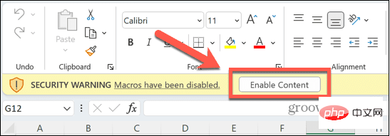 How to enable or disable macros in Excel
Apr 13, 2023 pm 10:43 PM
How to enable or disable macros in Excel
Apr 13, 2023 pm 10:43 PM
What are macros? A macro is a set of instructions that instruct Excel to perform an action or sequence of actions. They save you from performing repetitive tasks in Excel. In its simplest form, you can record a series of actions in Excel and save them as macros. Then, running your macro will perform the same sequence of operations as many times as you need. For example, you may want to insert multiple worksheets into your document. Inserting one at a time is not ideal, but a macro can insert any number of worksheets by repeating the same steps over and over. By using Visu
 How to embed a PDF document in an Excel worksheet
May 28, 2023 am 09:17 AM
How to embed a PDF document in an Excel worksheet
May 28, 2023 am 09:17 AM
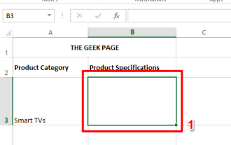
It is usually necessary to insert PDF documents into Excel worksheets. Just like a company's project list, we can instantly append text and character data to Excel cells. But what if you want to attach the solution design for a specific project to its corresponding data row? Well, people often stop and think. Sometimes thinking doesn't work either because the solution isn't simple. Dig deeper into this article to learn how to easily insert multiple PDF documents into an Excel worksheet, along with very specific rows of data. Example Scenario In the example shown in this article, we have a column called ProductCategory that lists a project name in each cell. Another column ProductSpeci
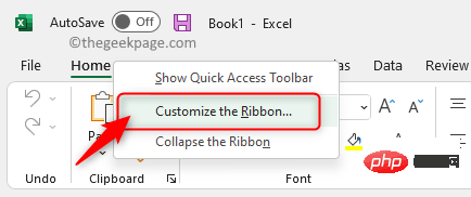 How to display the Developer tab in Microsoft Excel
Apr 14, 2023 pm 02:10 PM
How to display the Developer tab in Microsoft Excel
Apr 14, 2023 pm 02:10 PM
If you need to record or run macros, insert Visual Basic forms or ActiveX controls, or import/export XML files in MS Excel, you need the Developer tab in Excel for easy access. However, this developer tab does not appear by default, but you can add it to the ribbon by enabling it in Excel options. If you are working with macros and VBA and want to easily access them from the Ribbon, continue reading this article. Steps to enable Developer tab in Excel 1. Launch MS Excel application. Right-click anywhere on one of the top ribbon tabs and when
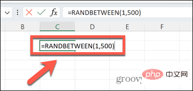 How to create a random number generator in Excel
Apr 14, 2023 am 09:46 AM
How to create a random number generator in Excel
Apr 14, 2023 am 09:46 AM
How to use RANDBETWEEN to generate random numbers in Excel If you want to generate random numbers within a specific range, the RANDBETWEEN function is a quick and easy way to do it. This allows you to generate random integers between any two values of your choice. Generate random numbers in Excel using RANDBETWEEN: Click the cell where you want the first random number to appear. Type =RANDBETWEEN(1,500) replacing "1" with the lowest random number you want to generate and "500" with