

Trading strategies and portfolio analysis using Python

We will measure the performance of trading strategies in this article. And will develop a simple momentum trading strategy that will use four asset classes: bonds, stocks, and real estate. These asset classes have low correlations, which makes them excellent risk-balancing options.

Momentum Trading Strategy
This strategy is based on momentum because traders and investors have long been aware of the impact of momentum, which can be seen in a wide range of market and time frame as seen. So we call it a momentum strategy. Trend following or time series momentum (TSM) is another name for using these strategies on a single instrument. We will create a basic momentum strategy and test it on TCS to see how it performs.
TSM Strategy Analysis
First, we will import some libraries
import numpy as np
 import pandas as pd
 import matplotlib.pyplot as plt
 import yfinance as yf
 import ffn
 %matplotlib inline
We build the basic momentum strategy function TSMStrategy. The function will return the expected performance via the logarithmic return of the time series, the time period of interest, and a Boolean variable for whether shorting is allowed.
def TSMStrategy(returns, period=1, shorts=False):
if shorts:
position = returns.rolling(period).mean().map(
lambda x: -1 if x <= 0 else 1)
else:
position = returns.rolling(period).mean().map(
lambda x: 0 if x <= 0 else 1)
performance = position.shift(1) * returns
return performance
 ticker = 'TCS'
 yftcs = yf.Ticker(ticker)
 data = yftcs.history(start='2005-01-01', end='2021-12-31')
 returns = np.log(data['Close'] / data['Close'].shift(1)).dropna()
 performance = TSMStrategy(returns, period=1, shorts=False).dropna()
 years = (performance.index.max() - performance.index.min()).days / 365
 perf_cum = np.exp(performance.cumsum())
 tot = perf_cum[-1] - 1
 ann = perf_cum[-1] ** (1 / years) - 1
 vol = performance.std() * np.sqrt(252)
 rfr = 0.02
 sharpe = (ann - rfr) / vol
 print(f"1-day TSM Strategy yields:" +
f"nt{tot*100:.2f}% total returns" +
f"nt{ann*100:.2f}% annual returns" +
f"nt{sharpe:.2f} Sharpe Ratio")
 tcs_ret = np.exp(returns.cumsum())
 b_tot = tcs_ret[-1] - 1
 b_ann = tcs_ret[-1] ** (1 / years) - 1
 b_vol = returns.std() * np.sqrt(252)
 b_sharpe = (b_ann - rfr) / b_vol
 print(f"Baseline Buy-and-Hold Strategy yields:" +
f"nt{b_tot*100:.2f}% total returns" +
f"nt{b_ann*100:.2f}% annual returns" +
f"nt{b_sharpe:.2f} Sharpe Ratio")The function output is as follows:
1-day TSM Strategy yields:
 -45.15% total returns
 -7.10% annual returns
 -0.17 Sharpe Ratio
 Baseline Buy-and-Hold Strategy yields:
 -70.15% total returns
 -13.78% annual returns
 -0.22 Sharpe Ratio
In terms of reasonable annualized returns, the 1-day TSM strategy is better than the buy and hold strategy. Because a 1-day lookback can contain many false trends, we tried different time periods to see how they compare. Here the model will be run in a loop for 3, 5, 15, 30 and 90 days.
 import matplotlib.gridspec as gridspec
 periods = [3, 5, 15, 30, 90]
 fig = plt.figure(figsize=(12, 10))
 gs = fig.add_gridspec(4, 4)
 ax0 = fig.add_subplot(gs[:2, :4])
 ax1 = fig.add_subplot(gs[2:, :2])
 ax2 = fig.add_subplot(gs[2:, 2:])
 ax0.plot((np.exp(returns.cumsum()) - 1) * 100, label=ticker, linestyle='-')
 perf_dict = {'tot_ret': {'buy_and_hold': (np.exp(returns.sum()) - 1)}}
 perf_dict['ann_ret'] = {'buy_and_hold': b_ann}
 perf_dict['sharpe'] = {'buy_and_hold': b_sharpe}
 for p in periods:
log_perf = TSMStrategy(returns, period=p, shorts=False)
perf = np.exp(log_perf.cumsum())
perf_dict['tot_ret'][p] = (perf[-1] - 1)
ann = (perf[-1] ** (1/years) - 1)
perf_dict['ann_ret'][p] = ann
vol = log_perf.std() * np.sqrt(252)
perf_dict['sharpe'][p] = (ann - rfr) / vol
ax0.plot((perf - 1) * 100, label=f'{p}-Day Mean')

 ax0.set_ylabel('Returns (%)')
 ax0.set_xlabel('Date')
 ax0.set_title('Cumulative Returns')
 ax0.grid()
 ax0.legend()
 _ = [ax1.bar(i, v * 100) for i, v in enumerate(perf_dict['ann_ret'].values())]
 ax1.set_xticks([i for i, k in enumerate(perf_dict['ann_ret'])])
 ax1.set_xticklabels([f'{k}-Day Mean'
if type(k) is int else ticker for
k in perf_dict['ann_ret'].keys()],
rotation=45)
 ax1.grid()
 ax1.set_ylabel('Returns (%)')
 ax1.set_xlabel('Strategy')
 ax1.set_title('Annual Returns')
 _ = [ax2.bar(i, v) for i, v in enumerate(perf_dict['sharpe'].values())]
 ax2.set_xticks([i for i, k in enumerate(perf_dict['sharpe'])])
 ax2.set_xticklabels([f'{k}-Day Mean'
if type(k) is int else ticker for
k in perf_dict['sharpe'].keys()],
rotation=45)
 ax2.grid()
 ax2.set_ylabel('Sharpe Ratio')
 ax2.set_xlabel('Strategy')
 ax2.set_title('Sharpe Ratio')
 plt.tight_layout()
 plt.show()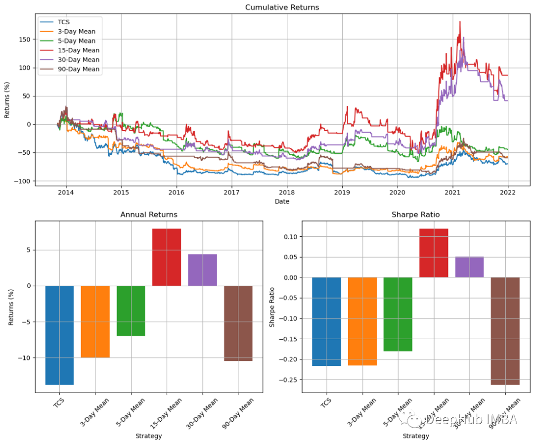
Looking at the results on the chart, we can see that the 15-day momentum indicator provides the best results. However, the results for other time periods are mixed. This shows that our strategy is not reliable. So we can also exit the trade by using a stop or trailing stop near the top, rather than doing it when the 15-day chart is down or flat.
PORTFOLIO ANALYSIS
So far we have created a trading strategy in Python. Below we will measure and plot common portfolio characteristics to facilitate our observation and analysis.
Portfolio Analysis
First, we will import some important libraries and observe the data execution.
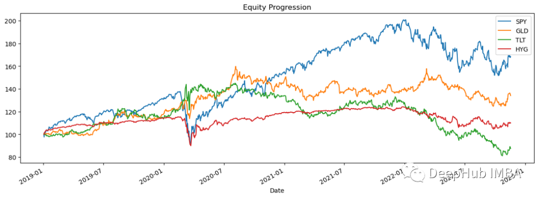
import pandas_datareader.data as web
 stocks = ['SPY','GLD','TLT','HYG']

 data = web.DataReader(stocks,data_source='yahoo',start='01/01/2019')['Adj Close']
 data.sort_index(ascending=True,inplace=True)
 perf = data.calc_stats()
 perf.plot()
Logarithmic Return
Logarithmic return is used to calculate exponential growth rate. Instead of calculating the percentage price change for each sub-period, we calculate the organic growth index for that period. First create a df that contains the log return of each stock price in the data, then we create a histogram for each log return.
 returns = data.to_log_returns().dropna()
 print(returns.head())


 Symbols SPY GLD TLT HYG
 Date
 2019-01-03 -0.024152 0.009025 0.011315 0.000494
 2019-01-04 0.032947 -0.008119 -0.011642 0.016644
 2019-01-07 0.007854 0.003453 -0.002953 0.009663
 2019-01-08 0.009351 -0.002712 -0.002631 0.006470
 2019-01-09 0.004663 0.006398 -0.001566 0.001193
The histograms are as follows:
ax = returns.hist(figsize=(20, 10),bins=30)
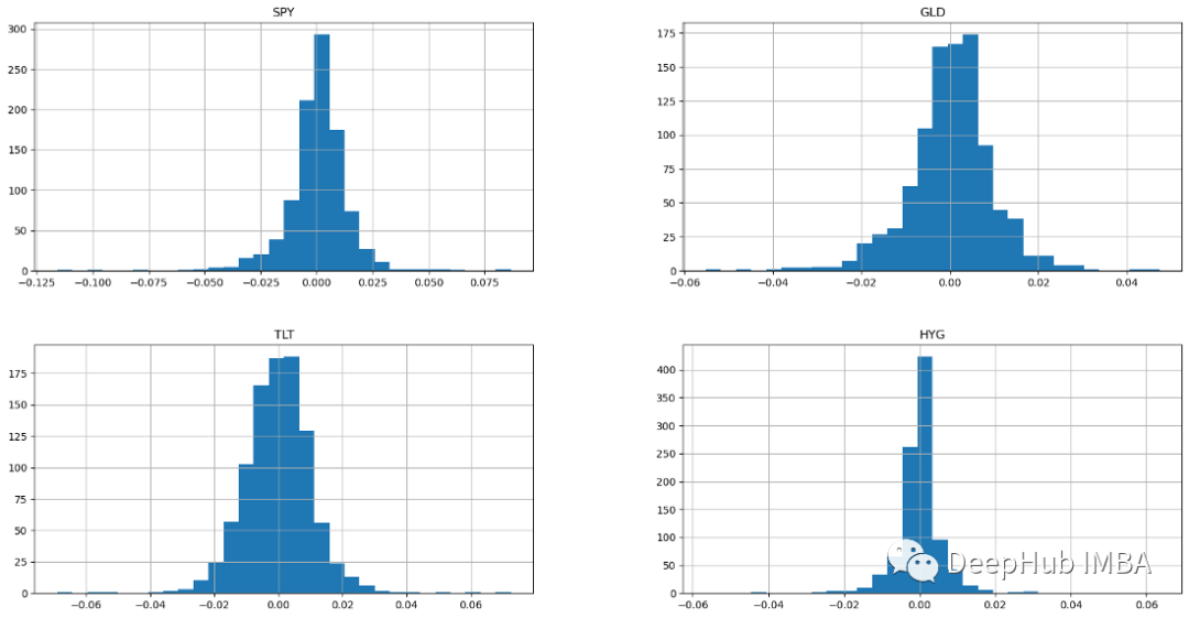
Histograms showing normal distribution for all four asset classes. A sample with a normal distribution has an arithmetic mean and an equal distribution above and below the mean (the normal distribution also known as the Gaussian distribution is symmetrical). If returns are normally distributed, more than 99% of returns are expected to fall within three standard deviations of the mean. These bell-shaped normal distribution characteristics allow analysts and investors to make better statistical inferences about a stock's expected returns and risks. Stocks with a bell curve are typically blue chips with low and predictable volatility.
Maximum retracement rate DRAWDOWN
DRAWDOWN refers to the value falling to a relative low. This is an important risk factor for investors to consider. Let us draw a visual representation of the decreasing strategy.
ffn.to_drawdown_series(data).plot(figsize=(15,10))
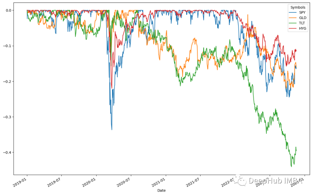
All four assets declined in the first half of 2020, with SPY experiencing the largest decline of 0.5%. Then, in the first half of 2020, all assets recovered immediately. This indicates a high asset recovery rate. These assets peaked around July 2020. Following this trend, all asset classes saw modest declines once the recovery peaked. According to the results, TLT will experience the largest decline of 0.5% in the second half of 2022 before recovering by early 2023.
MARKOWITZ Mean-variance optimization
In 1952, Markowitz (MARKOWITZ) proposed the mean-variance portfolio theory, also known as modern portfolio theory. Investors can use these concepts to construct a portfolio that maximizes expected returns based on a given level of risk. Based on the Markowitz method, we can generate an "optimal portfolio".
returns.calc_mean_var_weights().as_format('.2%')
 #结果
 SPY 46.60%
 GLD 53.40%
 TLT 0.00%
 HYG 0.00%
dtype: objectCorrelation Statistics
Correlation is a statistical method used to measure the relationship between securities. This information is best viewed using heat maps. Heatmaps allow us to see correlations between securities.
returns.plot_corr_heatmap()
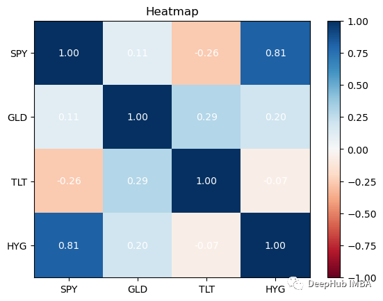
最好在你的投资组合中拥有相关性较低的资产。除了SPY与HYG,这四个资产类别的相关性都很低,这对我们的投资组合是不利的:因为如果拥有高度相关的不同资产组,即使你将风险分散在它们之间,从投资组合构建的角度来看,收益也会很少。
总结
通过分析和绘制的所有数据进行资产配置,可以建立一个投资组合,极大地改变基础投资的风险特征。还有很多我没有提到的,但可以帮助我们确定交易策略价值的起点。我们将在后续文章中添加更多的技术性能指标。
The above is the detailed content of Trading strategies and portfolio analysis using Python. For more information, please follow other related articles on the PHP Chinese website!

Hot AI Tools

Undresser.AI Undress
AI-powered app for creating realistic nude photos

AI Clothes Remover
Online AI tool for removing clothes from photos.

Undress AI Tool
Undress images for free

Clothoff.io
AI clothes remover

Video Face Swap
Swap faces in any video effortlessly with our completely free AI face swap tool!

Hot Article
Hot Tools

Notepad++7.3.1
Easy-to-use and free code editor

SublimeText3 Chinese version
Chinese version, very easy to use

Zend Studio 13.0.1
Powerful PHP integrated development environment

Dreamweaver CS6
Visual web development tools

SublimeText3 Mac version
God-level code editing software (SublimeText3)
Hot Topics


 PHP and Python: Different Paradigms Explained
Apr 18, 2025 am 12:26 AM
PHP and Python: Different Paradigms Explained
Apr 18, 2025 am 12:26 AM
PHP is mainly procedural programming, but also supports object-oriented programming (OOP); Python supports a variety of paradigms, including OOP, functional and procedural programming. PHP is suitable for web development, and Python is suitable for a variety of applications such as data analysis and machine learning.
 Choosing Between PHP and Python: A Guide
Apr 18, 2025 am 12:24 AM
Choosing Between PHP and Python: A Guide
Apr 18, 2025 am 12:24 AM
PHP is suitable for web development and rapid prototyping, and Python is suitable for data science and machine learning. 1.PHP is used for dynamic web development, with simple syntax and suitable for rapid development. 2. Python has concise syntax, is suitable for multiple fields, and has a strong library ecosystem.
 Python vs. JavaScript: The Learning Curve and Ease of Use
Apr 16, 2025 am 12:12 AM
Python vs. JavaScript: The Learning Curve and Ease of Use
Apr 16, 2025 am 12:12 AM
Python is more suitable for beginners, with a smooth learning curve and concise syntax; JavaScript is suitable for front-end development, with a steep learning curve and flexible syntax. 1. Python syntax is intuitive and suitable for data science and back-end development. 2. JavaScript is flexible and widely used in front-end and server-side programming.
 PHP and Python: A Deep Dive into Their History
Apr 18, 2025 am 12:25 AM
PHP and Python: A Deep Dive into Their History
Apr 18, 2025 am 12:25 AM
PHP originated in 1994 and was developed by RasmusLerdorf. It was originally used to track website visitors and gradually evolved into a server-side scripting language and was widely used in web development. Python was developed by Guidovan Rossum in the late 1980s and was first released in 1991. It emphasizes code readability and simplicity, and is suitable for scientific computing, data analysis and other fields.
 Can vs code run in Windows 8
Apr 15, 2025 pm 07:24 PM
Can vs code run in Windows 8
Apr 15, 2025 pm 07:24 PM
VS Code can run on Windows 8, but the experience may not be great. First make sure the system has been updated to the latest patch, then download the VS Code installation package that matches the system architecture and install it as prompted. After installation, be aware that some extensions may be incompatible with Windows 8 and need to look for alternative extensions or use newer Windows systems in a virtual machine. Install the necessary extensions to check whether they work properly. Although VS Code is feasible on Windows 8, it is recommended to upgrade to a newer Windows system for a better development experience and security.
 Can visual studio code be used in python
Apr 15, 2025 pm 08:18 PM
Can visual studio code be used in python
Apr 15, 2025 pm 08:18 PM
VS Code can be used to write Python and provides many features that make it an ideal tool for developing Python applications. It allows users to: install Python extensions to get functions such as code completion, syntax highlighting, and debugging. Use the debugger to track code step by step, find and fix errors. Integrate Git for version control. Use code formatting tools to maintain code consistency. Use the Linting tool to spot potential problems ahead of time.
 How to run sublime code python
Apr 16, 2025 am 08:48 AM
How to run sublime code python
Apr 16, 2025 am 08:48 AM
To run Python code in Sublime Text, you need to install the Python plug-in first, then create a .py file and write the code, and finally press Ctrl B to run the code, and the output will be displayed in the console.
 How to run python with notepad
Apr 16, 2025 pm 07:33 PM
How to run python with notepad
Apr 16, 2025 pm 07:33 PM
Running Python code in Notepad requires the Python executable and NppExec plug-in to be installed. After installing Python and adding PATH to it, configure the command "python" and the parameter "{CURRENT_DIRECTORY}{FILE_NAME}" in the NppExec plug-in to run Python code in Notepad through the shortcut key "F6".
