
 Backend Development
Python Tutorial
How to use Python to implement the PSO algorithm to solve the TSP problem?
Backend Development
Python Tutorial
How to use Python to implement the PSO algorithm to solve the TSP problem?
How to use Python to implement the PSO algorithm to solve the TSP problem?

PSO Algorithm
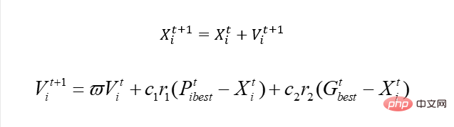
Before we start, let’s talk about the basic PSO algorithm. The core is just one:

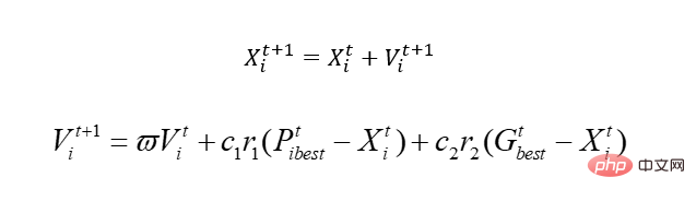
Let’s explain this formula, and you’ll understand.
Old rules let us assume that there is an equation y=sin(x1) cos(x2)
The PSO algorithm achieves our optimization by simulating bird migration. I won’t say how this came about. Okay, let’s talk about this core.
In the equation we just had, there are two variables, x1, x2. Because it is a simulated bird, in order to realize the blind method, the concept of speed is introduced here. Naturally, x is our feasible domain, which is the solution space. By changing the speed, x is moved, that is, the value of x is changed. Among them, Pbest represents the optimal solution in the location where the bird has walked, and Gbest represents the optimal solution of the entire population. What do you mean, that is to say, as it moves, this bird may move to a worse position, because unlike genetics, it will be killed if it is bad, but this one will not. Of course, there are many local issues involved, which we will not discuss here. No algorithm is perfect, and this one is right.
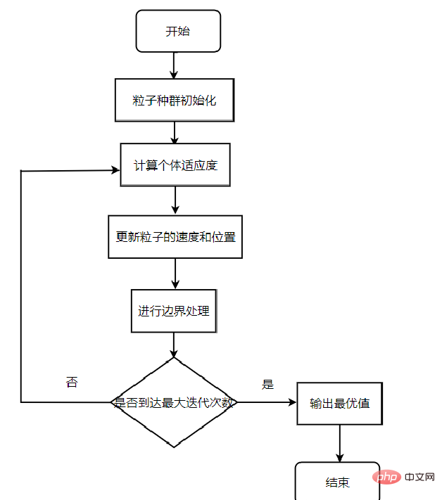
Algorithm process
The main process of the algorithm:
The first step: Initialize the random position and speed of the particle swarm, and set the number of iterations.
Step 2: Calculate the fitness value of each particle.
Step 3: For each particle, compare its fitness value with the fitness value of the best position pbest i experienced. If it is better, use it as the current individual optimal position. .
Step 4: For each particle, compare its fitness value with the fitness value of the best position gbestg experienced globally. If it is better, use it as the current global optimal position. .
Step 5: Optimize the speed and position of the particles according to the speed and position formulas to update the particle position.
Step 6: If the end condition is not reached (usually the maximum number of cycles or the minimum error requirement), return to the second step
Advantages:
PSO algorithm has no crossover and mutation operations and relies on particle speed to complete the search. In the iterative evolution, only the optimal particles pass information to other particles, so the search speed is fast.
PSO algorithm has memory, and the historical best position of the particle group can be memorized and passed to other particles.
There are fewer parameters that need to be adjusted, the structure is simple, and it is easy to implement in engineering.
Adopts real number encoding, which is directly determined by the solution of the problem. The number of variables in the problem solution is directly used as the dimension of the particle.
Disadvantages:
Lacks dynamic adjustment of speed and easily falls into local optimum, resulting in low convergence accuracy and difficulty in convergence.
Cannot effectively solve discrete and combinatorial optimization problems.
Parameter control, for different problems, how to choose appropriate parameters to achieve optimal results.
Cannot effectively solve some non-cartesian coordinate system description problems,
Simple implementation
ok, let’s take a look at the simplest implementation:
import numpy as np
import random
class PSO_model:
def __init__(self,w,c1,c2,r1,r2,N,D,M):
self.w = w # 惯性权值
self.c1=c1
self.c2=c2
self.r1=r1
self.r2=r2
self.N=N # 初始化种群数量个数
self.D=D # 搜索空间维度
self.M=M # 迭代的最大次数
self.x=np.zeros((self.N,self.D)) #粒子的初始位置
self.v=np.zeros((self.N,self.D)) #粒子的初始速度
self.pbest=np.zeros((self.N,self.D)) #个体最优值初始化
self.gbest=np.zeros((1,self.D)) #种群最优值
self.p_fit=np.zeros(self.N)
self.fit=1e8 #初始化全局最优适应度
# 目标函数,也是适应度函数(求最小化问题)
def function(self,x):
A = 10
x1=x[0]
x2=x[1]
Z = 2 * A + x1 ** 2 - A * np.cos(2 * np.pi * x1) + x2 ** 2 - A * np.cos(2 * np.pi * x2)
return Z
# 初始化种群
def init_pop(self):
for i in range(self.N):
for j in range(self.D):
self.x[i][j] = random.random()
self.v[i][j] = random.random()
self.pbest[i] = self.x[i] # 初始化个体的最优值
aim=self.function(self.x[i]) # 计算个体的适应度值
self.p_fit[i]=aim # 初始化个体的最优位置
if aim < self.fit: # 对个体适应度进行比较,计算出最优的种群适应度
self.fit = aim
self.gbest = self.x[i]
# 更新粒子的位置与速度
def update(self):
for t in range(self.M): # 在迭代次数M内进行循环
for i in range(self.N): # 对所有种群进行一次循环
aim=self.function(self.x[i]) # 计算一次目标函数的适应度
if aim<self.p_fit[i]: # 比较适应度大小,将小的负值给个体最优
self.p_fit[i]=aim
self.pbest[i]=self.x[i]
if self.p_fit[i]<self.fit: # 如果是个体最优再将和全体最优进行对比
self.gbest=self.x[i]
self.fit = self.p_fit[i]
for i in range(self.N): # 更新粒子的速度和位置
self.v[i]=self.w*self.v[i]+self.c1*self.r1*(self.pbest[i]-self.x[i])+ self.c2*self.r2*(self.gbest-self.x[i])
self.x[i]=self.x[i]+self.v[i]
print("最优值:",self.fit,"位置为:",self.gbest)
if __name__ == '__main__':
# w,c1,c2,r1,r2,N,D,M参数初始化
w=random.random()
c1=c2=2#一般设置为2
r1=0.7
r2=0.5
N=30
D=2
M=200
pso_object=PSO_model(w,c1,c2,r1,r2,N,D,M)#设置初始权值
pso_object.init_pop()
pso_object.update()Solution TSP
Data representation
First of all, using PSO is actually similar to our previous use of genetics. We still use a matrix to represent the population, and a matrix to represent the distance between cities. .
      # 群体的初始化和路径的初始化
        self.population = np.array([0] * self.num_pop * self.num).reshape(
            self.num_pop, self.num)
        self.fitness = [0] * self.num_pop
        """
        计算城市的距离,我们用矩阵表示城市间的距离
        """
self.__matrix_distance = self.__matrix_dis()Difference
What is the biggest difference from our original PSO? In fact, it is simple and related to our speed of updating. When we have a continuous problem, it is actually like this:
Similarly, we can use X to represent the city number, but obviously we cannot use this solution to update the speed.
At this time, if we want to update the speed, we need to use a new solution. So this solution is actually the X update using the genetic algorithm. To put it bluntly, the reason why we need speed is to update X and make X move in a good direction. Now it is no longer possible to simply use speed update, so we are updating X anyway, so why not just choose a solution that can update this X well? Therefore, genetics can be used directly here. Our speed update is based on Pbest and Gbest, and then "learned" according to a certain weight. In this way, this V has a "characteristic" of Pbest and Gbest. So if that's the case, then when I directly imitate genetic crossover and cross it with Best, can't I learn some corresponding "features"?
    def cross_1(self, path, best_path):
        r1 = np.random.randint(self.num)
        r2 = np.random.randint(self.num)
        while r2 == r1:
            r2 = np.random.randint(self.num)
        left, right = min(r1, r2), max(r1, r2)
        cross = best_path[left:right + 1]
        for i in range(right - left + 1):
            for k in range(self.num):
                if path[k] == cross[i]:
                    path[k:self.num - 1] = path[k + 1:self.num]
                    path[-1] = 0
        path[self.num - right + left - 1:self.num] = cross
return pathAt the same time we can still introduce mutations.
    def mutation(self,path):
        r1 = np.random.randint(self.num)
        r2 = np.random.randint(self.num)
        while r2 == r1:
            r2 = np.random.randint(self.num)
        path[r1],path[r2] = path[r2],path[r1]
return pathComplete code
ok, now let’s see the complete code:
import numpy as np
import matplotlib.pyplot as plt
class HybridPsoTSP(object):
    def __init__(self ,data ,num_pop=200):
        self.num_pop = num_pop  # 群体个数
        self.data = data        # 城市坐标
        self.num =len(data)     # 城市个数
        # 群体的初始化和路径的初始化
        self.population = np.array([0] * self.num_pop * self.num).reshape(
            self.num_pop, self.num)
        self.fitness = [0] * self.num_pop
        """
        计算城市的距离,我们用矩阵表示城市间的距离
        """
        self.__matrix_distance = self.__matrix_dis()
    def __matrix_dis(self):
        """
        计算14个城市的距离,将这些距离用矩阵存起来
        :return:
        """
        res = np.zeros((self.num, self.num))
        for i in range(self.num):
            for j in range(i + 1, self.num):
                res[i, j] = np.linalg.norm(self.data[i, :] - self.data[j, :])
                res[j, i] = res[i, j]
        return res
    def cross_1(self, path, best_path):
        r1 = np.random.randint(self.num)
        r2 = np.random.randint(self.num)
        while r2 == r1:
            r2 = np.random.randint(self.num)
        left, right = min(r1, r2), max(r1, r2)
        cross = best_path[left:right + 1]
        for i in range(right - left + 1):
            for k in range(self.num):
                if path[k] == cross[i]:
                    path[k:self.num - 1] = path[k + 1:self.num]
                    path[-1] = 0
        path[self.num - right + left - 1:self.num] = cross
        return path
    def mutation(self,path):
        r1 = np.random.randint(self.num)
        r2 = np.random.randint(self.num)
        while r2 == r1:
            r2 = np.random.randint(self.num)
        path[r1],path[r2] = path[r2],path[r1]
        return path
    def comp_fit(self, one_path):
        """
        计算,咱们这个路径的长度,例如A-B-C-D
        :param one_path:
        :return:
        """
        res = 0
        for i in range(self.num - 1):
            res += self.__matrix_distance[one_path[i], one_path[i + 1]]
        res += self.__matrix_distance[one_path[-1], one_path[0]]
        return res
    def out_path(self, one_path):
        """
        输出我们的路径顺序
        :param one_path:
        :return:
        """
        res = str(one_path[0] + 1) + '-->'
        for i in range(1, self.num):
            res += str(one_path[i] + 1) + '-->'
        res += str(one_path[0] + 1) + '\n'
        print(res)
    def init_population(self):
        """
        初始化种群
        :return:
        """
        rand_ch = np.array(range(self.num))
        for i in range(self.num_pop):
            np.random.shuffle(rand_ch)
            self.population[i, :] = rand_ch
            self.fitness[i] = self.comp_fit(rand_ch)
def main(data, max_n=200, num_pop=200):
    Path_short = HybridPsoTSP(data, num_pop=num_pop)  # 混合粒子群算法类
    Path_short.init_population()  # 初始化种群
    # 初始化路径绘图
    fig, ax = plt.subplots()
    x = data[:, 0]
    y = data[:, 1]
    ax.scatter(x, y, linewidths=0.1)
    for i, txt in enumerate(range(1, len(data) + 1)):
        ax.annotate(txt, (x[i], y[i]))
    res0 = Path_short.population[0]
    x0 = x[res0]
    y0 = y[res0]
    for i in range(len(data) - 1):
        plt.quiver(x0[i], y0[i], x0[i + 1] - x0[i], y0[i + 1] - y0[i], color='r', width=0.005, angles='xy', scale=1,
                   scale_units='xy')
    plt.quiver(x0[-1], y0[-1], x0[0] - x0[-1], y0[0] - y0[-1], color='r', width=0.005, angles='xy', scale=1,
               scale_units='xy')
    plt.show()
    print('初始染色体的路程: ' + str(Path_short.fitness[0]))
    # 存储个体极值的路径和距离
    best_P_population = Path_short.population.copy()
    best_P_fit = Path_short.fitness.copy()
    min_index = np.argmin(Path_short.fitness)
    # 存储当前种群极值的路径和距离
    best_G_population = Path_short.population[min_index, :]
    best_G_fit = Path_short.fitness[min_index]
    # 存储每一步迭代后的最优路径和距离
    best_population = [best_G_population]
    best_fit = [best_G_fit]
    # 复制当前群体进行交叉变异
    x_new = Path_short.population.copy()
    for i in range(max_n):
        # 更新当前的个体极值
        for j in range(num_pop):
            if Path_short.fitness[j] < best_P_fit[j]:
                best_P_fit[j] = Path_short.fitness[j]
                best_P_population[j, :] = Path_short.population[j, :]
        # 更新当前种群的群体极值
        min_index = np.argmin(Path_short.fitness)
        best_G_population = Path_short.population[min_index, :]
        best_G_fit = Path_short.fitness[min_index]
        # 更新每一步迭代后的全局最优路径和解
        if best_G_fit < best_fit[-1]:
            best_fit.append(best_G_fit)
            best_population.append(best_G_population)
        else:
            best_fit.append(best_fit[-1])
            best_population.append(best_population[-1])
        # 将每个个体与个体极值和当前的群体极值进行交叉
        for j in range(num_pop):
            # 与个体极值交叉
            x_new[j, :] = Path_short.cross_1(x_new[j, :], best_P_population[j, :])
            fit = Path_short.comp_fit(x_new[j, :])
            # 判断是否保留
            if fit < Path_short.fitness[j]:
                Path_short.population[j, :] = x_new[j, :]
                Path_short.fitness[j] = fit
            # 与当前极值交叉
            x_new[j, :] = Path_short.cross_1(x_new[j, :], best_G_population)
            fit = Path_short.comp_fit(x_new[j, :])
            if fit < Path_short.fitness[j]:
                Path_short.population[j, :] = x_new[j, :]
                Path_short.fitness[j] = fit
            # 变异
            x_new[j, :] = Path_short.mutation(x_new[j, :])
            fit = Path_short.comp_fit(x_new[j, :])
            if fit <= Path_short.fitness[j]:
                Path_short.population[j] = x_new[j, :]
                Path_short.fitness[j] = fit
        if (i + 1) % 20 == 0:
            print('第' + str(i + 1) + '步后的最短的路程: ' + str(Path_short.fitness[min_index]))
            print('第' + str(i + 1) + '步后的最优路径:')
            Path_short.out_path(Path_short.population[min_index, :])  # 显示每一步的最优路径
    Path_short.best_population = best_population
    Path_short.best_fit = best_fit
    return Path_short  # 返回结果类
if __name__ == '__main__':
    data = np.array([16.47, 96.10, 16.47, 94.44, 20.09, 92.54,
                     22.39, 93.37, 25.23, 97.24, 22.00, 96.05, 20.47, 97.02,
                     17.20, 96.29, 16.30, 97.38, 14.05, 98.12, 16.53, 97.38,
                     21.52, 95.59, 19.41, 97.13, 20.09, 92.55]).reshape((14, 2))
main(data)初始染色体的路程: 71.30211569672313
第20步后的最短的路程: 29.340520066994223
第20步后的最优路径:
9-->10-->1-->2-->14-->3-->4-->5-->6-->12-->7-->13-->8-->11-->9
第40步后的最短的路程: 29.340520066994223
第40步后的最优路径:
9-->10-->1-->2-->14-->3-->4-->5-->6-->12-->7-->13-->8-->11-->9
第60步后的最短的路程: 29.340520066994223
第60步后的最优路径:
9-->10-->1-->2-->14-->3-->4-->5-->6-->12-->7-->13-->8-->11-->9
第80步后的最短的路程: 29.340520066994223
第80步后的最优路径:
9-->10-->1-->2-->14-->3-->4-->5-->6-->12-->7-->13-->8-->11-->9
第100步后的最短的路程: 29.340520066994223
第100步后的最优路径:
9-->10-->1-->2-->14-->3-->4-->5-->6-->12-->7-->13-->8-->11-->9
第120步后的最短的路程: 29.340520066994223
第120步后的最优路径:
9-->10-->1-->2-->14-->3-->4-->5-->6-->12-->7-->13-->8-->11-->9
第140步后的最短的路程: 29.340520066994223
第140步后的最优路径:
9-->10-->1-->2-->14-->3-->4-->5-->6-->12-->7-->13-->8-->11-->9
第160步后的最短的路程: 29.340520066994223
第160步后的最优路径:
9-->10-->1-->2-->14-->3-->4-->5-->6-->12-->7-->13-->8-->11-->9
第180步后的最短的路程: 29.340520066994223
第180步后的最优路径:
9-->10-->1-->2-->14-->3-->4-->5-->6-->12-->7-->13-->8-->11-->9
第200步后的最短的路程: 29.340520066994223
第200步后的最优路径:
9-->10-->1-->2-->14-->3-->4-->5-->6-->12-->7-->13-->8-->11-->9
可以看到收敛速度还是很快的。
特点分析
ok,到目前为止的话,我们介绍了两个算法去解决TSP或者是优化问题。我们来分析一下,这些算法有什么特点,为啥可以达到我们需要的优化效果。其实不管是遗传还是PSO,你其实都可以发现,有一个东西,我们可以暂且叫它环境压力。我们通过物竞天择,或者鸟类迁移,进行模拟寻优。而之所以需要这样做,是因为我们指定了一个规则,在我们的规则之下。我们让模拟的种群有一种压力去靠拢,其中物竞天择和鸟类迁移只是我们的一种手段,去应对这样的“压力”。所以的对于这种算法而言,最核心的点就两个:
设计环境压力
我们需要做优化问题,所以我们必须要能够让我们的解往那个方向走,需要一个驱动,需要一个压力。因此我们需要设计这样的一个环境,在遗传算法,粒子群算法是通过种群当中的生存,来进行设计的它的压力是我们的目标函数。由种群和目标函数(目标指标)构成了一个环境和压力。
设计压力策略
之后的话,我们设计好了一个环境和压力,那么未来应对这种压力,我们需要去设计一种策略,来应付这种压力。遗传算法是通过PUA自己,也就是种群的优胜略汰。PSO是通过学习,学习种群的优秀粒子和过去自己家的优秀“祖先”来应对这种压力的。
强化学习
所以的话,我们是否可以使用别的方案来实现这种优化效果。,在强化学习的算法框架里面的话,我们明确的知道了为什么他们可以实现优化,是环境压力+压力策略。恰好咱们强化学习是有环境的,适应函数和环境恰好可以组成环境+压力。本身的算法收敛过程就是我们的压力策略。所以我们完全是可以直接使用强化学习进行这个处理的。那么在这里咱们就来使用强化学习在下一篇文章当中。
The above is the detailed content of How to use Python to implement the PSO algorithm to solve the TSP problem?. For more information, please follow other related articles on the PHP Chinese website!

Hot AI Tools

Undresser.AI Undress
AI-powered app for creating realistic nude photos

AI Clothes Remover
Online AI tool for removing clothes from photos.

Undress AI Tool
Undress images for free

Clothoff.io
AI clothes remover

Video Face Swap
Swap faces in any video effortlessly with our completely free AI face swap tool!

Hot Article
Hot Tools

Notepad++7.3.1
Easy-to-use and free code editor

SublimeText3 Chinese version
Chinese version, very easy to use

Zend Studio 13.0.1
Powerful PHP integrated development environment

Dreamweaver CS6
Visual web development tools

SublimeText3 Mac version
God-level code editing software (SublimeText3)
Hot Topics


 PHP and Python: Different Paradigms Explained
Apr 18, 2025 am 12:26 AM
PHP and Python: Different Paradigms Explained
Apr 18, 2025 am 12:26 AM
PHP is mainly procedural programming, but also supports object-oriented programming (OOP); Python supports a variety of paradigms, including OOP, functional and procedural programming. PHP is suitable for web development, and Python is suitable for a variety of applications such as data analysis and machine learning.
 Choosing Between PHP and Python: A Guide
Apr 18, 2025 am 12:24 AM
Choosing Between PHP and Python: A Guide
Apr 18, 2025 am 12:24 AM
PHP is suitable for web development and rapid prototyping, and Python is suitable for data science and machine learning. 1.PHP is used for dynamic web development, with simple syntax and suitable for rapid development. 2. Python has concise syntax, is suitable for multiple fields, and has a strong library ecosystem.
 PHP and Python: A Deep Dive into Their History
Apr 18, 2025 am 12:25 AM
PHP and Python: A Deep Dive into Their History
Apr 18, 2025 am 12:25 AM
PHP originated in 1994 and was developed by RasmusLerdorf. It was originally used to track website visitors and gradually evolved into a server-side scripting language and was widely used in web development. Python was developed by Guidovan Rossum in the late 1980s and was first released in 1991. It emphasizes code readability and simplicity, and is suitable for scientific computing, data analysis and other fields.
 Python vs. JavaScript: The Learning Curve and Ease of Use
Apr 16, 2025 am 12:12 AM
Python vs. JavaScript: The Learning Curve and Ease of Use
Apr 16, 2025 am 12:12 AM
Python is more suitable for beginners, with a smooth learning curve and concise syntax; JavaScript is suitable for front-end development, with a steep learning curve and flexible syntax. 1. Python syntax is intuitive and suitable for data science and back-end development. 2. JavaScript is flexible and widely used in front-end and server-side programming.
 How to run sublime code python
Apr 16, 2025 am 08:48 AM
How to run sublime code python
Apr 16, 2025 am 08:48 AM
To run Python code in Sublime Text, you need to install the Python plug-in first, then create a .py file and write the code, and finally press Ctrl B to run the code, and the output will be displayed in the console.
 Can vs code run in Windows 8
Apr 15, 2025 pm 07:24 PM
Can vs code run in Windows 8
Apr 15, 2025 pm 07:24 PM
VS Code can run on Windows 8, but the experience may not be great. First make sure the system has been updated to the latest patch, then download the VS Code installation package that matches the system architecture and install it as prompted. After installation, be aware that some extensions may be incompatible with Windows 8 and need to look for alternative extensions or use newer Windows systems in a virtual machine. Install the necessary extensions to check whether they work properly. Although VS Code is feasible on Windows 8, it is recommended to upgrade to a newer Windows system for a better development experience and security.
 Where to write code in vscode
Apr 15, 2025 pm 09:54 PM
Where to write code in vscode
Apr 15, 2025 pm 09:54 PM
Writing code in Visual Studio Code (VSCode) is simple and easy to use. Just install VSCode, create a project, select a language, create a file, write code, save and run it. The advantages of VSCode include cross-platform, free and open source, powerful features, rich extensions, and lightweight and fast.
 Can visual studio code be used in python
Apr 15, 2025 pm 08:18 PM
Can visual studio code be used in python
Apr 15, 2025 pm 08:18 PM
VS Code can be used to write Python and provides many features that make it an ideal tool for developing Python applications. It allows users to: install Python extensions to get functions such as code completion, syntax highlighting, and debugging. Use the debugger to track code step by step, find and fix errors. Integrate Git for version control. Use code formatting tools to maintain code consistency. Use the Linting tool to spot potential problems ahead of time.
