
 Technology peripherals
AI
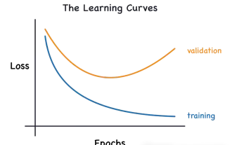
What can training and validation metric graphs tell us in machine learning?
Technology peripherals
AI
What can training and validation metric graphs tell us in machine learning?
What can training and validation metric graphs tell us in machine learning?

In this article, we will summarize the possible situations of training and verification and introduce what kind of information these charts can provide us.
Let’s start with some simple code. The following code establishes a basic training process framework.
from sklearn.model_selection import train_test_split<br>from sklearn.datasets import make_classification<br>import torch<br>from torch.utils.data import Dataset, DataLoader<br>import torch.optim as torch_optim<br>import torch.nn as nn<br>import torch.nn.functional as F<br>import numpy as np<br>import matplotlib.pyplot as pltclass MyCustomDataset(Dataset):<br>def __init__(self, X, Y, scale=False):<br>self.X = torch.from_numpy(X.astype(np.float32))<br>self.y = torch.from_numpy(Y.astype(np.int64))<br><br>def __len__(self):<br>return len(self.y)<br><br>def __getitem__(self, idx):<br>return self.X[idx], self.y[idx]def get_optimizer(model, lr=0.001, wd=0.0):<br>parameters = filter(lambda p: p.requires_grad, model.parameters())<br>optim = torch_optim.Adam(parameters, lr=lr, weight_decay=wd)<br>return optimdef train_model(model, optim, train_dl, loss_func):<br># Ensure the model is in Training mode<br>model.train()<br>total = 0<br>sum_loss = 0<br>for x, y in train_dl:<br>batch = y.shape[0]<br># Train the model for this batch worth of data<br>logits = model(x)<br># Run the loss function. We will decide what this will be when we call our Training Loop<br>loss = loss_func(logits, y)<br># The next 3 lines do all the PyTorch back propagation goodness<br>optim.zero_grad()<br>loss.backward()<br>optim.step()<br># Keep a running check of our total number of samples in this epoch<br>total += batch<br># And keep a running total of our loss<br>sum_loss += batch*(loss.item())<br>return sum_loss/total<br>def train_loop(model, train_dl, valid_dl, epochs, loss_func, lr=0.1, wd=0):<br>optim = get_optimizer(model, lr=lr, wd=wd)<br>train_loss_list = []<br>val_loss_list = []<br>acc_list = []<br>for i in range(epochs): <br>loss = train_model(model, optim, train_dl, loss_func)<br># After training this epoch, keep a list of progress of <br># the loss of each epoch <br>train_loss_list.append(loss)<br>val, acc = val_loss(model, valid_dl, loss_func)<br># Likewise for the validation loss and accuracy<br>val_loss_list.append(val)<br>acc_list.append(acc)<br>print("training loss: %.5f valid loss: %.5f accuracy: %.5f" % (loss, val, acc))<br><br>return train_loss_list, val_loss_list, acc_list<br>def val_loss(model, valid_dl, loss_func):<br># Put the model into evaluation mode, not training mode<br>model.eval()<br>total = 0<br>sum_loss = 0<br>correct = 0<br>batch_count = 0<br>for x, y in valid_dl:<br>batch_count += 1<br>current_batch_size = y.shape[0]<br>logits = model(x)<br>loss = loss_func(logits, y)<br>sum_loss += current_batch_size*(loss.item())<br>total += current_batch_size<br># All of the code above is the same, in essence, to<br># Training, so see the comments there<br># Find out which of the returned predictions is the loudest<br># of them all, and that's our prediction(s)<br>preds = logits.sigmoid().argmax(1)<br># See if our predictions are right<br>correct += (preds == y).float().mean().item()<br>return sum_loss/total, correct/batch_count<br>def view_results(train_loss_list, val_loss_list, acc_list):<br>plt.rcParams["figure.figsize"] = (15, 5)<br>plt.figure()<br>epochs = np.arange(0, len(train_loss_list)) plt.subplot(1, 2, 1)<br>plt.plot(epochs-0.5, train_loss_list)<br>plt.plot(epochs, val_loss_list)<br>plt.title('model loss')<br>plt.ylabel('loss')<br>plt.xlabel('epoch')<br>plt.legend(['train', 'val', 'acc'], loc = 'upper left')<br><br>plt.subplot(1, 2, 2)<br>plt.plot(acc_list)<br>plt.title('accuracy')<br>plt.ylabel('accuracy')<br>plt.xlabel('epoch')<br>plt.legend(['train', 'val', 'acc'], loc = 'upper left')<br>plt.show()<br><br>def get_data_train_and_show(model, batch_size=128, n_samples=10000, n_classes=2, n_features=30, val_size=0.2, epochs=20, lr=0.1, wd=0, break_it=False):<br># We'll make a fictitious dataset, assuming all relevant<br># EDA / Feature Engineering has been done and this is our <br># resultant data<br>X, y = make_classification(n_samples=n_samples, n_classes=n_classes, n_features=n_features, n_informative=n_features, n_redundant=0, random_state=1972)<br><br>if break_it: # Specifically mess up the data<br>X = np.random.rand(n_samples,n_features)<br>X_train, X_val, y_train, y_val = train_test_split(X, y, test_size=val_size, random_state=1972) train_ds = MyCustomDataset(X_train, y_train)<br>valid_ds = MyCustomDataset(X_val, y_val)<br>train_dl = DataLoader(train_ds, batch_size=batch_size, shuffle=True)<br>valid_dl = DataLoader(valid_ds, batch_size=batch_size, shuffle=True) train_loss_list, val_loss_list, acc_list = train_loop(model, train_dl, valid_dl, epochs=epochs, loss_func=F.cross_entropy, lr=lr, wd=wd)<br>view_results(train_loss_list, val_loss_list, acc_list)The above code is very simple, it is a basic process of obtaining data, training, and verification. Let’s get to the point.
Scenario 1 - Model seems to learn, but performs poorly in validation or accuracy
Regardless of hyperparameters, model Train loss slowly decreases, but Val loss does not decrease, and Its Accuracy does not indicate that it is learning anything.
For example, in this case, the accuracy of binary classification hovers around 50%.
class Scenario_1_Model_1(nn.Module):<br>def __init__(self, in_features=30, out_features=2):<br>super().__init__()<br>self.lin1 = nn.Linear(in_features, out_features)<br>def forward(self, x):<br>x = self.lin1(x)<br>return x<br>get_data_train_and_show(Scenario_1_Model_1(), lr=0.001, break_it=True)

There is not enough information in the data to allow 'learning', and the training data may not contain enough information to allow the model to 'learn'.
In this case (the training data in the code is random data), this means that it cannot learn anything of substance.
The data must have enough information to learn from. EDA and feature engineering are key! Models learn what can be learned, rather than making up things that don’t exist.
Scenario 2 - Training, validation and accuracy curves are all very unstable
For example, the following code: lr=0.1, bs=128
class Scenario_2_Model_1(nn.Module):<br>def __init__(self, in_features=30, out_features=2):<br>super().__init__()<br>self.lin1 = nn.Linear(in_features, out_features)<br>def forward(self, x):<br>x = self.lin1(x)<br>return x<br>get_data_train_and_show(Scenario_2_Model_1(), lr=0.1)

"Learning rate is too high" or "batch is too small" You can try to reduce the learning rate from 0.1 to 0.001, which means that it will not "bounce", but will decrease smoothly.
get_data_train_and_show(Scenario_1_Model_1(), lr=0.001)

In addition to lowering the learning rate, increasing the batch size will also make it smoother.
get_data_train_and_show(Scenario_1_Model_1(), lr=0.001, batch_size=256)

Scenario 3 - Training loss is close to zero, accuracy looks good, but validation does not go down, and also goes up
class Scenario_3_Model_1(nn.Module):<br>def __init__(self, in_features=30, out_features=2):<br>super().__init__()<br>self.lin1 = nn.Linear(in_features, 50)<br>self.lin2 = nn.Linear(50, 150)<br>self.lin3 = nn.Linear(150, 50)<br>self.lin4 = nn.Linear(50, out_features)<br>def forward(self, x):<br>x = F.relu(self.lin1(x))<br>x = F.relu(self.lin2(x))<br>x = F.relu(self.lin3(x))<br>x = self.lin4(x)<br>return x<br>get_data_train_and_show(Scenario_3_Model_1(), lr=0.001)

This is definitely overfitting: the training loss is low and the accuracy is high, while the verification loss and training loss are getting larger and larger, which are both classic overfitting indicators.
Fundamentally speaking, your model learning ability is too strong. It remembers the training data too well, which means it also cannot generalize to new data.
The first thing we can try is to reduce the complexity of the model.
class Scenario_3_Model_2(nn.Module):<br>def __init__(self, in_features=30, out_features=2):<br>super().__init__()<br>self.lin1 = nn.Linear(in_features, 50)<br>self.lin2 = nn.Linear(50, out_features)<br>def forward(self, x):<br>x = F.relu(self.lin1(x))<br>x = self.lin2(x)<br>return x<br>get_data_train_and_show(Scenario_3_Model_2(), lr=0.001)

This makes it better, and L2 weight decay regularization can be introduced to make it even better again (for shallower models).
get_data_train_and_show(Scenario_3_Model_2(), lr=0.001, wd=0.02)

If we want to maintain the depth and size of the model, we can try using dropout (for deeper models).
class Scenario_3_Model_3(nn.Module):<br>def __init__(self, in_features=30, out_features=2):<br>super().__init__()<br>self.lin1 = nn.Linear(in_features, 50)<br>self.lin2 = nn.Linear(50, 150)<br>self.lin3 = nn.Linear(150, 50)<br>self.lin4 = nn.Linear(50, out_features)<br>self.drops = nn.Dropout(0.4)<br>def forward(self, x):<br>x = F.relu(self.lin1(x))<br>x = self.drops(x)<br>x = F.relu(self.lin2(x))<br>x = self.drops(x)<br>x = F.relu(self.lin3(x))<br>x = self.drops(x)<br>x = self.lin4(x)<br>return x<br>get_data_train_and_show(Scenario_3_Model_3(), lr=0.001)

场景 4 - 训练和验证表现良好,但准确度没有提高
lr = 0.001,bs = 128(默认,分类类别= 5
class Scenario_4_Model_1(nn.Module):<br>def __init__(self, in_features=30, out_features=2):<br>super().__init__()<br>self.lin1 = nn.Linear(in_features, 2)<br>self.lin2 = nn.Linear(2, out_features)<br>def forward(self, x):<br>x = F.relu(self.lin1(x))<br>x = self.lin2(x)<br>return x<br>get_data_train_and_show(Scenario_4_Model_1(out_features=5), lr=0.001, n_classes=5)

没有足够的学习能力:模型中的其中一层的参数少于模型可能输出中的类。 在这种情况下,当有 5 个可能的输出类时,中间的参数只有 2 个。
这意味着模型会丢失信息,因为它不得不通过一个较小的层来填充它,因此一旦层的参数再次扩大,就很难恢复这些信息。
所以需要记录层的参数永远不要小于模型的输出大小。
class Scenario_4_Model_2(nn.Module):<br>def __init__(self, in_features=30, out_features=2):<br>super().__init__()<br>self.lin1 = nn.Linear(in_features, 50)<br>self.lin2 = nn.Linear(50, out_features)<br>def forward(self, x):<br>x = F.relu(self.lin1(x))<br>x = self.lin2(x)<br>return x<br>get_data_train_and_show(Scenario_4_Model_2(out_features=5), lr=0.001, n_classes=5)

总结
以上就是一些常见的训练、验证时的曲线的示例,希望你在遇到相同情况时可以快速定位并且改进。
The above is the detailed content of What can training and validation metric graphs tell us in machine learning?. For more information, please follow other related articles on the PHP Chinese website!

Hot AI Tools

Undresser.AI Undress
AI-powered app for creating realistic nude photos

AI Clothes Remover
Online AI tool for removing clothes from photos.

Undress AI Tool
Undress images for free

Clothoff.io
AI clothes remover

Video Face Swap
Swap faces in any video effortlessly with our completely free AI face swap tool!

Hot Article
Hot Tools

Notepad++7.3.1
Easy-to-use and free code editor

SublimeText3 Chinese version
Chinese version, very easy to use

Zend Studio 13.0.1
Powerful PHP integrated development environment

Dreamweaver CS6
Visual web development tools

SublimeText3 Mac version
God-level code editing software (SublimeText3)
Hot Topics


 This article will take you to understand SHAP: model explanation for machine learning
Jun 01, 2024 am 10:58 AM
This article will take you to understand SHAP: model explanation for machine learning
Jun 01, 2024 am 10:58 AM
In the fields of machine learning and data science, model interpretability has always been a focus of researchers and practitioners. With the widespread application of complex models such as deep learning and ensemble methods, understanding the model's decision-making process has become particularly important. Explainable AI|XAI helps build trust and confidence in machine learning models by increasing the transparency of the model. Improving model transparency can be achieved through methods such as the widespread use of multiple complex models, as well as the decision-making processes used to explain the models. These methods include feature importance analysis, model prediction interval estimation, local interpretability algorithms, etc. Feature importance analysis can explain the decision-making process of a model by evaluating the degree of influence of the model on the input features. Model prediction interval estimate
 Identify overfitting and underfitting through learning curves
Apr 29, 2024 pm 06:50 PM
Identify overfitting and underfitting through learning curves
Apr 29, 2024 pm 06:50 PM
This article will introduce how to effectively identify overfitting and underfitting in machine learning models through learning curves. Underfitting and overfitting 1. Overfitting If a model is overtrained on the data so that it learns noise from it, then the model is said to be overfitting. An overfitted model learns every example so perfectly that it will misclassify an unseen/new example. For an overfitted model, we will get a perfect/near-perfect training set score and a terrible validation set/test score. Slightly modified: "Cause of overfitting: Use a complex model to solve a simple problem and extract noise from the data. Because a small data set as a training set may not represent the correct representation of all data." 2. Underfitting Heru
 Slow Cellular Data Internet Speeds on iPhone: Fixes
May 03, 2024 pm 09:01 PM
Slow Cellular Data Internet Speeds on iPhone: Fixes
May 03, 2024 pm 09:01 PM
Facing lag, slow mobile data connection on iPhone? Typically, the strength of cellular internet on your phone depends on several factors such as region, cellular network type, roaming type, etc. There are some things you can do to get a faster, more reliable cellular Internet connection. Fix 1 – Force Restart iPhone Sometimes, force restarting your device just resets a lot of things, including the cellular connection. Step 1 – Just press the volume up key once and release. Next, press the Volume Down key and release it again. Step 2 – The next part of the process is to hold the button on the right side. Let the iPhone finish restarting. Enable cellular data and check network speed. Check again Fix 2 – Change data mode While 5G offers better network speeds, it works better when the signal is weaker
 Tesla robots work in factories, Musk: The degree of freedom of hands will reach 22 this year!
May 06, 2024 pm 04:13 PM
Tesla robots work in factories, Musk: The degree of freedom of hands will reach 22 this year!
May 06, 2024 pm 04:13 PM
The latest video of Tesla's robot Optimus is released, and it can already work in the factory. At normal speed, it sorts batteries (Tesla's 4680 batteries) like this: The official also released what it looks like at 20x speed - on a small "workstation", picking and picking and picking: This time it is released One of the highlights of the video is that Optimus completes this work in the factory, completely autonomously, without human intervention throughout the process. And from the perspective of Optimus, it can also pick up and place the crooked battery, focusing on automatic error correction: Regarding Optimus's hand, NVIDIA scientist Jim Fan gave a high evaluation: Optimus's hand is the world's five-fingered robot. One of the most dexterous. Its hands are not only tactile
 The vitality of super intelligence awakens! But with the arrival of self-updating AI, mothers no longer have to worry about data bottlenecks
Apr 29, 2024 pm 06:55 PM
The vitality of super intelligence awakens! But with the arrival of self-updating AI, mothers no longer have to worry about data bottlenecks
Apr 29, 2024 pm 06:55 PM
I cry to death. The world is madly building big models. The data on the Internet is not enough. It is not enough at all. The training model looks like "The Hunger Games", and AI researchers around the world are worrying about how to feed these data voracious eaters. This problem is particularly prominent in multi-modal tasks. At a time when nothing could be done, a start-up team from the Department of Renmin University of China used its own new model to become the first in China to make "model-generated data feed itself" a reality. Moreover, it is a two-pronged approach on the understanding side and the generation side. Both sides can generate high-quality, multi-modal new data and provide data feedback to the model itself. What is a model? Awaker 1.0, a large multi-modal model that just appeared on the Zhongguancun Forum. Who is the team? Sophon engine. Founded by Gao Yizhao, a doctoral student at Renmin University’s Hillhouse School of Artificial Intelligence.
 Implementing Machine Learning Algorithms in C++: Common Challenges and Solutions
Jun 03, 2024 pm 01:25 PM
Implementing Machine Learning Algorithms in C++: Common Challenges and Solutions
Jun 03, 2024 pm 01:25 PM
Common challenges faced by machine learning algorithms in C++ include memory management, multi-threading, performance optimization, and maintainability. Solutions include using smart pointers, modern threading libraries, SIMD instructions and third-party libraries, as well as following coding style guidelines and using automation tools. Practical cases show how to use the Eigen library to implement linear regression algorithms, effectively manage memory and use high-performance matrix operations.
 The U.S. Air Force showcases its first AI fighter jet with high profile! The minister personally conducted the test drive without interfering during the whole process, and 100,000 lines of code were tested for 21 times.
May 07, 2024 pm 05:00 PM
The U.S. Air Force showcases its first AI fighter jet with high profile! The minister personally conducted the test drive without interfering during the whole process, and 100,000 lines of code were tested for 21 times.
May 07, 2024 pm 05:00 PM
Recently, the military circle has been overwhelmed by the news: US military fighter jets can now complete fully automatic air combat using AI. Yes, just recently, the US military’s AI fighter jet was made public for the first time and the mystery was unveiled. The full name of this fighter is the Variable Stability Simulator Test Aircraft (VISTA). It was personally flown by the Secretary of the US Air Force to simulate a one-on-one air battle. On May 2, U.S. Air Force Secretary Frank Kendall took off in an X-62AVISTA at Edwards Air Force Base. Note that during the one-hour flight, all flight actions were completed autonomously by AI! Kendall said - "For the past few decades, we have been thinking about the unlimited potential of autonomous air-to-air combat, but it has always seemed out of reach." However now,
 Five schools of machine learning you don't know about
Jun 05, 2024 pm 08:51 PM
Five schools of machine learning you don't know about
Jun 05, 2024 pm 08:51 PM
Machine learning is an important branch of artificial intelligence that gives computers the ability to learn from data and improve their capabilities without being explicitly programmed. Machine learning has a wide range of applications in various fields, from image recognition and natural language processing to recommendation systems and fraud detection, and it is changing the way we live. There are many different methods and theories in the field of machine learning, among which the five most influential methods are called the "Five Schools of Machine Learning". The five major schools are the symbolic school, the connectionist school, the evolutionary school, the Bayesian school and the analogy school. 1. Symbolism, also known as symbolism, emphasizes the use of symbols for logical reasoning and expression of knowledge. This school of thought believes that learning is a process of reverse deduction, through existing
