
 Topics
excel
Practical Excel skills sharing: Explore the 'little secrets' hidden in automatic sorting
Topics
excel
Practical Excel skills sharing: Explore the 'little secrets' hidden in automatic sorting
Practical Excel skills sharing: Explore the 'little secrets' hidden in automatic sorting

It is said that there are hidden secrets in Excel. The MAX function for finding the maximum value can be used for searching, and the LOOKUP function used for searching can round the data... Even Excel’s automatic sorting, which everyone seems to know, has many hidden secrets. The “little secret” we don’t know. Today we will explore these "little secrets" hidden in automatic sorting.

1. Expanding the selection
"Teacher Miao, why is my sorting wrong? ", hearing Xiaobai's call, I walked over quickly.
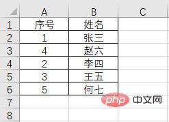
"Look, I just want to sort this table by serial number." (As shown in Figure 1)
Picture 1
"But after finishing the arrangement, it turned out like this. The numbers were arranged, but the names did not change with the numbers. The names and serial numbers were all messed up."
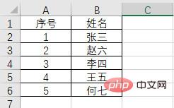
Figure 2
"When this problem occurs, you must have not expanded the selection. Usually when you select a column of data in the table for sorting, such a window will pop up", as shown in Figure 3.
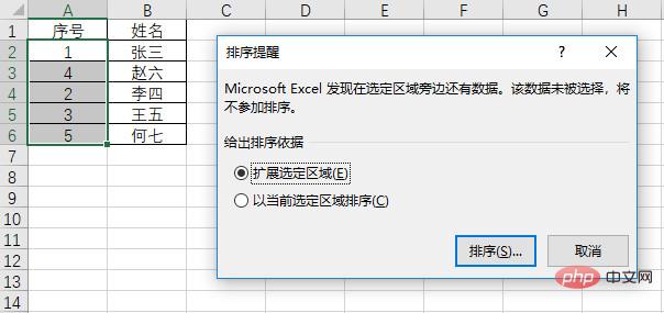
Figure 3
Generally, by default, "Extend selected area" is selected and then click "Sort" to complete the overall sorting. Or before sorting, select the entire data area and then click Sort to complete the overall sorting and this reminder window will not pop up again.
2. Primary and secondary keywords for multi-column sorting
When we perform multi-column sorting, we often encounter such a category Question: If there are two columns of data that need to be sorted, how do we distinguish between primary and secondary? As shown in Figure 4, the following table needs to be sorted first by "department" and then by "region".
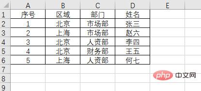
Figure 4
At this time, do not click the "Ascending" and "Descending" buttons directly, but click the "Sort" button first, as shown in Figure 5.
Figure 5
After opening, as shown in Figure 6.
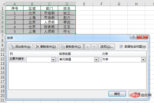
Figure 6
We add all the sorting conditions that need to be set into the setting box. After adding a condition, click "Add Condition" to add the third 2 conditions, as shown in Figure 7.
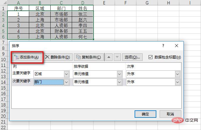
Figure 7
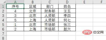
After completing the settings, click "OK", and you will get a table sorted first by "Area" and then by "Department", such as As shown in Figure 8.
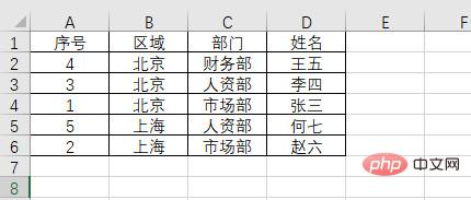
Figure 8
Since what we are starting to do is a table sorted by "department" first and then by "region", we want to achieve this effect. , you need to change the primary and secondary keywords. How to change it? Just click the small triangle in the sorting window, as shown in Figure 9.
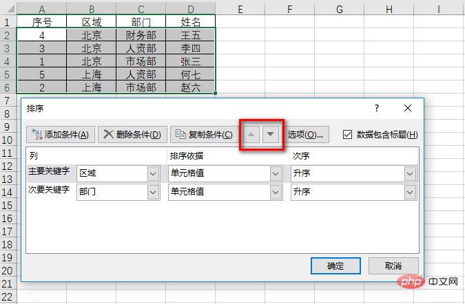
Figure 9
Here we select the "Main Keywords" row, click the "Down" arrow, and finally "OK" to achieve what we originally wanted. desired sorting effect. As shown in Figure 10.
Picture 10
3. Sort by color
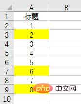
"Teacher Miao, I touched again I have a question." Xiaobai sent another table. She said: "I have some cells marked with a yellow background. Now I want to separate the yellow parts from the ones without a background. What should I do? I copy and insert I've been doing this for a long time."
"It's sorting. If you copy and insert one by one like this, you won't be able to finish it tomorrow."
"Can this also be sorted? You need to use Function?"
"No. In fact, this function is in the sorting, but you don't pay attention to it."
said and opened her table, as shown in Figure 11.
Picture 11
In the "Data" tab, click "Sort" to enter the "Sort" setting box. Since our data has titles, we need to check "Data contains titles". Then set the "Sort by" to "Cell Color". In "Order", you can choose whether to sort colored data or uncolored data first according to your needs. Here we set the colored cells to be ranked at the top. As shown in Figure 12.
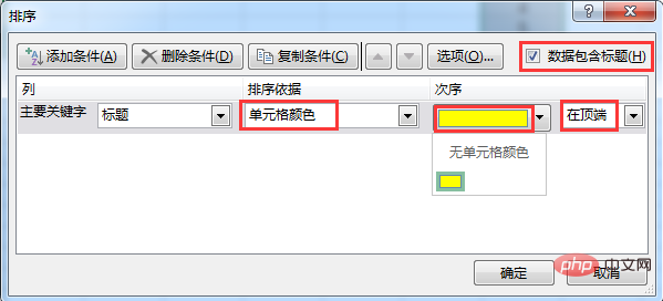
Figure 12
After clicking "OK", you can separate the colored cells from the uncolored cells, as shown in Figure 13
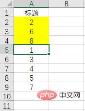
Figure 13
In fact, in the "Sort by", there are other options, such as sorting by font color, etc. You can try it yourself. As shown in Figure 14
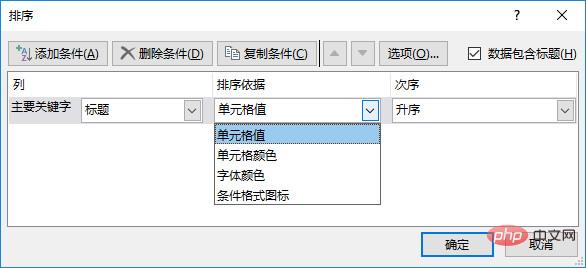
Figure 14
4. Custom sorting
In fact, In addition to the sorting mentioned above, there is another function that is most easily overlooked by everyone, which is "custom sorting", which is also hidden in the "sorting" interface. As shown in Figure 15.

Figure 15
We can sort numbers and text, but what if we need to sort specific content? For example, the list of branches in various locations, the sequence of positions and leaders within the company, etc. They all have a specific order and often need to be produced or arranged in daily work. The picture below shows the order of departments in our company. Suppose it is disrupted. How can we restore it to the normal order?
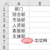
Figure 16
At this time, it is definitely impossible to use ordinary ascending and descending order, so this sequence needs to be set by ourselves. In the sorting settings box, click "Custom Sequence" to open the custom sequence settings box, as shown in Figure 17.
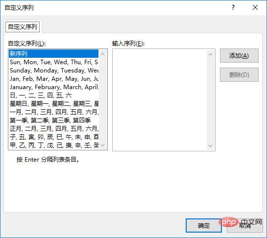
Figure 17
In the "Input Sequence" area, create the sequence we need. For example, if we want to make a sequence of departments, in the "Input Sequence" area, enter the department names in sequence, and press the Enter key to separate each department name. After completing the input, click "Add" and the sequence just added will appear in the "Custom Sequence" on the left. As shown in Figure 18.
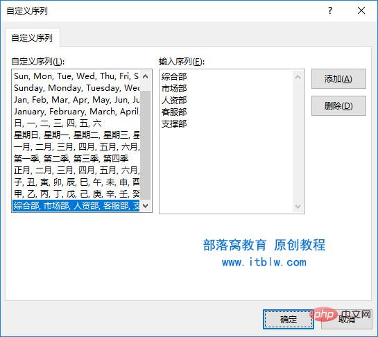
Figure 18
After the setting is completed, just select "Custom Sequence" in the sorting setting box, click on the set department sequence, and the data can be The order we set is sorted. As shown in GIF19.

GIF19
Extended functions: In addition to the usage mentioned above, using custom sequence sorting, department names can also appear in a drop-down manner, as shown in GIF20 Show.
GIF20
With this function, as long as you write down the first department name or the first leader name, you can complete the entry of the sequence through the drop-down method. No more worries about confusing department names or missing leader names! How is it? Is it useful?
Related learning recommendations: excel tutorial
The above is the detailed content of Practical Excel skills sharing: Explore the 'little secrets' hidden in automatic sorting. For more information, please follow other related articles on the PHP Chinese website!

Hot AI Tools

Undresser.AI Undress
AI-powered app for creating realistic nude photos

AI Clothes Remover
Online AI tool for removing clothes from photos.

Undress AI Tool
Undress images for free

Clothoff.io
AI clothes remover

Video Face Swap
Swap faces in any video effortlessly with our completely free AI face swap tool!

Hot Article
Hot Tools

Notepad++7.3.1
Easy-to-use and free code editor

SublimeText3 Chinese version
Chinese version, very easy to use

Zend Studio 13.0.1
Powerful PHP integrated development environment

Dreamweaver CS6
Visual web development tools

SublimeText3 Mac version
God-level code editing software (SublimeText3)
Hot Topics


 What should I do if the frame line disappears when printing in Excel?
Mar 21, 2024 am 09:50 AM
What should I do if the frame line disappears when printing in Excel?
Mar 21, 2024 am 09:50 AM
If when opening a file that needs to be printed, we will find that the table frame line has disappeared for some reason in the print preview. When encountering such a situation, we must deal with it in time. If this also appears in your print file If you have questions like this, then join the editor to learn the following course: What should I do if the frame line disappears when printing a table in Excel? 1. Open a file that needs to be printed, as shown in the figure below. 2. Select all required content areas, as shown in the figure below. 3. Right-click the mouse and select the "Format Cells" option, as shown in the figure below. 4. Click the “Border” option at the top of the window, as shown in the figure below. 5. Select the thin solid line pattern in the line style on the left, as shown in the figure below. 6. Select "Outer Border"
 How to filter more than 3 keywords at the same time in excel
Mar 21, 2024 pm 03:16 PM
How to filter more than 3 keywords at the same time in excel
Mar 21, 2024 pm 03:16 PM
Excel is often used to process data in daily office work, and it is often necessary to use the "filter" function. When we choose to perform "filtering" in Excel, we can only filter up to two conditions for the same column. So, do you know how to filter more than 3 keywords at the same time in Excel? Next, let me demonstrate it to you. The first method is to gradually add the conditions to the filter. If you want to filter out three qualifying details at the same time, you first need to filter out one of them step by step. At the beginning, you can first filter out employees with the surname "Wang" based on the conditions. Then click [OK], and then check [Add current selection to filter] in the filter results. The steps are as follows. Similarly, perform filtering separately again
 How to change excel table compatibility mode to normal mode
Mar 20, 2024 pm 08:01 PM
How to change excel table compatibility mode to normal mode
Mar 20, 2024 pm 08:01 PM
In our daily work and study, we copy Excel files from others, open them to add content or re-edit them, and then save them. Sometimes a compatibility check dialog box will appear, which is very troublesome. I don’t know Excel software. , can it be changed to normal mode? So below, the editor will bring you detailed steps to solve this problem, let us learn together. Finally, be sure to remember to save it. 1. Open a worksheet and display an additional compatibility mode in the name of the worksheet, as shown in the figure. 2. In this worksheet, after modifying the content and saving it, the dialog box of the compatibility checker always pops up. It is very troublesome to see this page, as shown in the figure. 3. Click the Office button, click Save As, and then
 How to type subscript in excel
Mar 20, 2024 am 11:31 AM
How to type subscript in excel
Mar 20, 2024 am 11:31 AM
eWe often use Excel to make some data tables and the like. Sometimes when entering parameter values, we need to superscript or subscript a certain number. For example, mathematical formulas are often used. So how do you type the subscript in Excel? ?Let’s take a look at the detailed steps: 1. Superscript method: 1. First, enter a3 (3 is superscript) in Excel. 2. Select the number "3", right-click and select "Format Cells". 3. Click "Superscript" and then "OK". 4. Look, the effect is like this. 2. Subscript method: 1. Similar to the superscript setting method, enter "ln310" (3 is the subscript) in the cell, select the number "3", right-click and select "Format Cells". 2. Check "Subscript" and click "OK"
 How to set superscript in excel
Mar 20, 2024 pm 04:30 PM
How to set superscript in excel
Mar 20, 2024 pm 04:30 PM
When processing data, sometimes we encounter data that contains various symbols such as multiples, temperatures, etc. Do you know how to set superscripts in Excel? When we use Excel to process data, if we do not set superscripts, it will make it more troublesome to enter a lot of our data. Today, the editor will bring you the specific setting method of excel superscript. 1. First, let us open the Microsoft Office Excel document on the desktop and select the text that needs to be modified into superscript, as shown in the figure. 2. Then, right-click and select the "Format Cells" option in the menu that appears after clicking, as shown in the figure. 3. Next, in the “Format Cells” dialog box that pops up automatically
 How to use the iif function in excel
Mar 20, 2024 pm 06:10 PM
How to use the iif function in excel
Mar 20, 2024 pm 06:10 PM
Most users use Excel to process table data. In fact, Excel also has a VBA program. Apart from experts, not many users have used this function. The iif function is often used when writing in VBA. It is actually the same as if The functions of the functions are similar. Let me introduce to you the usage of the iif function. There are iif functions in SQL statements and VBA code in Excel. The iif function is similar to the IF function in the excel worksheet. It performs true and false value judgment and returns different results based on the logically calculated true and false values. IF function usage is (condition, yes, no). IF statement and IIF function in VBA. The former IF statement is a control statement that can execute different statements according to conditions. The latter
 Where to set excel reading mode
Mar 21, 2024 am 08:40 AM
Where to set excel reading mode
Mar 21, 2024 am 08:40 AM
In the study of software, we are accustomed to using excel, not only because it is convenient, but also because it can meet a variety of formats needed in actual work, and excel is very flexible to use, and there is a mode that is convenient for reading. Today I brought For everyone: where to set the excel reading mode. 1. Turn on the computer, then open the Excel application and find the target data. 2. There are two ways to set the reading mode in Excel. The first one: In Excel, there are a large number of convenient processing methods distributed in the Excel layout. In the lower right corner of Excel, there is a shortcut to set the reading mode. Find the pattern of the cross mark and click it to enter the reading mode. There is a small three-dimensional mark on the right side of the cross mark.
 How to insert excel icons into PPT slides
Mar 26, 2024 pm 05:40 PM
How to insert excel icons into PPT slides
Mar 26, 2024 pm 05:40 PM
1. Open the PPT and turn the page to the page where you need to insert the excel icon. Click the Insert tab. 2. Click [Object]. 3. The following dialog box will pop up. 4. Click [Create from file] and click [Browse]. 5. Select the excel table to be inserted. 6. Click OK and the following page will pop up. 7. Check [Show as icon]. 8. Click OK.
