

The 4 most practical pivot table tips for learning Excel pivot tables

I didn’t learn much about functions, so I focused on pivot tables. Pivot tables don’t disappoint, there are always little things that can solve big statistical problems. The 4 home remedies here are just that.

The so-called folk remedies refer to prescriptions that are rarely seen in normal times but have special effects on specific situations. Today we share with you 4 "recipes" for pivot tables.
Recipe 1: Null value processing
When we perform data pivot on a set of data, we often encounter the situation where the corresponding data of a certain field in the value area is blank. . In the past, many partners made manual modifications. In fact, you can customize the blank display to 0 through a pivot table. (Note: Only for blanks in the value area!)
Example:
The purchase quantity of the screen 300*220 item in the first quarter is blank, and now the data needs to be pivoted and summarized.
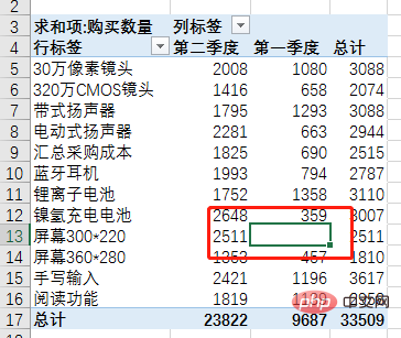
After completing the pivot, we see that cell C13 is blank.
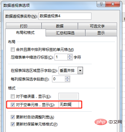
Click the PivotTable, right-click the mouse, and select [PivotTable Options].

Open the [Pivot Table Options] dialog box, check [Display for blank cells] in [Layout and Format], and at the same time, in the edit bar on the right Enter "No data" in the box.
#After clicking OK, all the blank spaces in the PivotTable will be filled with "No Data" characters.
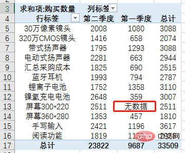
Note: Here we can fill the blanks with any text, numbers or symbols by definition.
Recipe 2: Ranking
In daily work, it is often necessary to rank the data after completing the data pivot. Many partners use the rank function to rank. In fact, pivot tables come with a ranking function, so there is no need for sorting or functions at all.
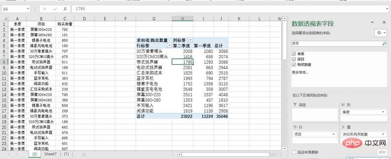
Still taking purchasing data as an example, now we have completed the data pivot.
Select the pivot table, right-click the mouse, select [Value Display Mode], and select [Sort Descending] in the submenu.
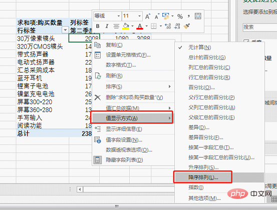
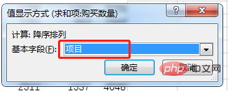
Select items as the basic field for sorting and click [OK].
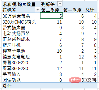
Finally we saw that the original purchase data information turned into ranking information.
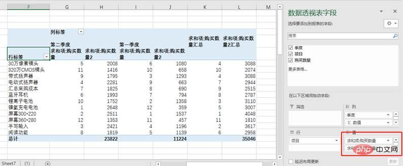
If we need to retain purchase data and ranking information at the same time, we only need to add the purchase quantity in the value field again.
Recipe Three: Create Worksheets in Batch
Batch creation is a task that is often encountered in daily life, such as creating branches, months , quarterly and other worksheets. If the number is small, we can create it one by one manually. What if the number is large? In fact, you can create worksheets in batches through pivot tables.
Example: Now we need to create a worksheet for 4 quarters.
First enter the header quarter and the names of the four quarters in the table.
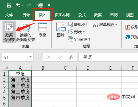
Then select the data in column A and click [Pivot Table] in the [Insert] tab.
In the [Create PivotTable] dialog box that opens, select the location of the PivotTable as an existing worksheet.

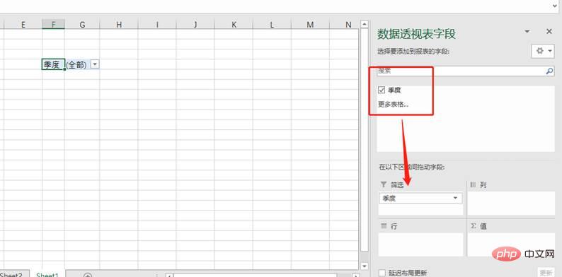
After confirmation, drag the [Quarter] field to the filter box.
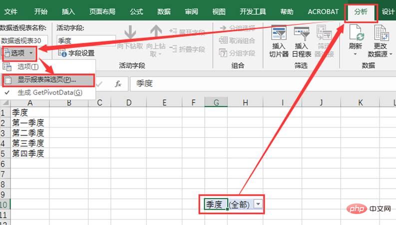
Click the PivotTable, and then click [Options] - [Show Report Filter Page] in the [Analysis] tab.
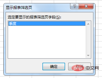
#The [Show Report Filter Page] dialog box appears, click OK directly, and we can see the batch-created worksheets.
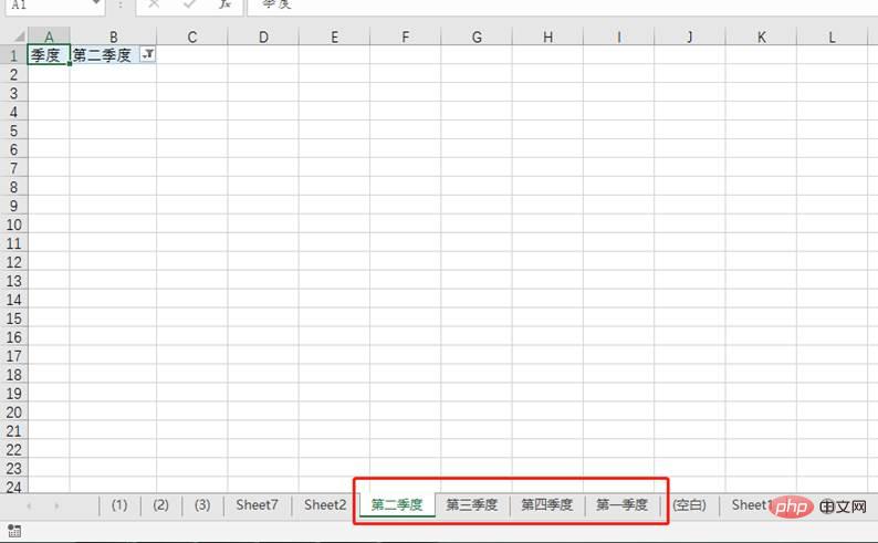
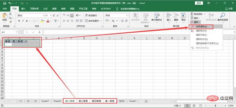
Select all the worksheets created, then select the unnecessary data in the table in any worksheet, and select "Start" - " Clear"-"Clear All" to complete the batch creation of worksheets.
Is not it simple?
Note: Worksheets created in batches are automatically sorted by worksheet name. For example, for the first to fourth quarters here, the created worksheets are second, third, fourth, and first quarter in order. If you want to create a worksheet in quarterly order, change the input to Arabic numerals, such as the 1st, 2nd, 3rd, 4th, etc. quarters. If you want to create worksheets in the order of the names you enter, an easy way is to add Arabic numerals 1, 2, 3, etc. in front of each name when inputting, and the worksheets will be created in the order of input.
Recipe 4: Group statistics by new fields
It is also a common thing to group data by new fields for statistics. For example, there are no months or quarters in the data, but your boss asks you to make statistics on a monthly or quarterly basis; there are no first-, second-, or third-class products in the data, but your boss asks you to make statistics on first-, second-, and third-class products. For this kind of statistics of original data according to newly specified fields, it can be very easily implemented using a pivot table.
Give two examples.
Example 1: Group statistics by date
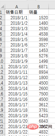
The data source is sales registered by day. Now we want to count sales by month and quarter.
(1) Select all the data and insert the pivot table.
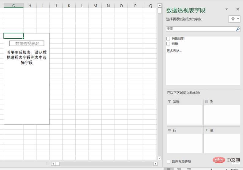
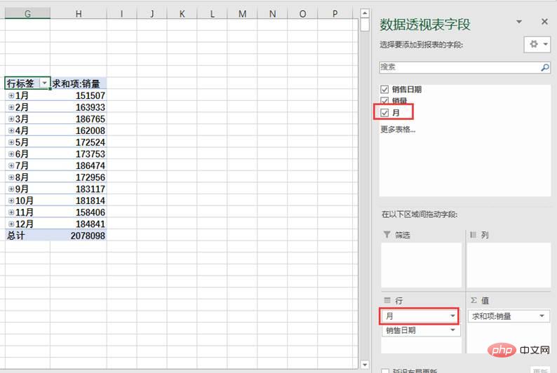
(2) Drag the "Sales Date" field into the row area, Excel will automatically add a "Month" field (requires the 2016 version), and the row in the right pivot table Tags are displayed by month. (Note: If you are using an earlier version, you need to set the "Quarter" field as shown below. Only after adding the "Month" field can statistics be calculated on a monthly basis.) Then drag "Sales" into the value area.
(3) Next we implement quarterly statistics through grouping settings. Right-click on any data under the pivot table row label and select the "Combine" command (you can also click [Analyze] - [Group Field] or [Group Selection]) to open the [Combine] dialog box. You can see that the two step sizes "day" and "month" have been selected.
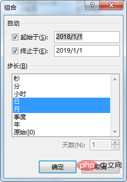
#Start at and end at data will be automatically generated based on the data source, don’t worry about it.
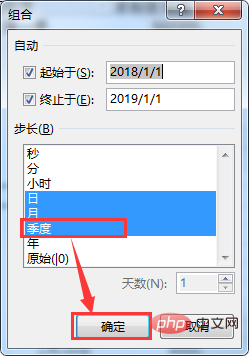
(4) Click "Quarter" and then OK.
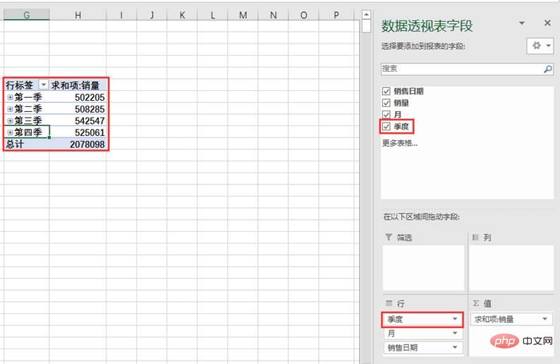
# (5) You can see that the "Quarter" field has been added to the pivot table field. In the pivot table on the left, click the  symbol to collapse the data and achieve quarterly statistics.
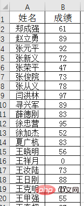
Example 2: Score statistics by stages
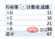
The following table shows the mathematics scores of a certain class, with only two fields: name and score. . Now we need to count the number of people in each stage, 60-79, 80-100.
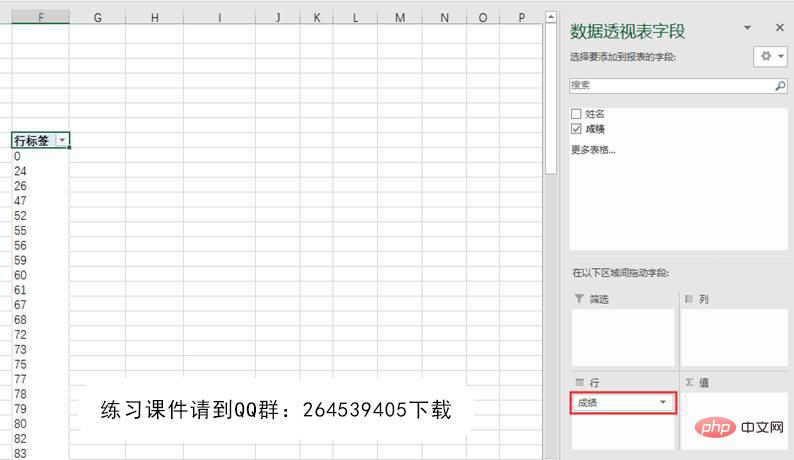
(1) Same as above, first create a pivot table.

(2) Drag the "Grade" field into the row area. At this time, a column of fractional values appears below the row labels of the left pivot table.
(3) Right-click on any score under the pivot table row label and select the "Combine" command to open the Combination dialog box.
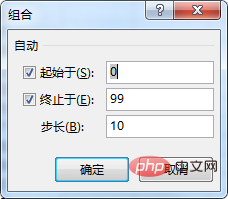
# (4) Now modify the starting value, ending value, and step size as needed. The settings start at 60 and end at 100 in steps of 20, as follows.
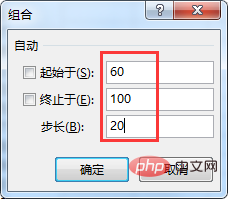
(5) After clicking "OK", the row label changes to the three fractional segments we need.

(6) Drag the "Grade" field to the value area to implement headcount statistics. For example, there are 11 people who failed.
(7) If you want to further see the names at each stage, you can drag the "Name" field into the row area.
If you want to segment more freely without being restricted by the step size, you can change the approach in step (3). For example, select 0-59, right-click, select "Combine", generate "Data Group 1", select "Data Group 1", enter "D" in the edit bar, change "Data Group 1" to "D", this It is the grade D stage; select 60-79, right-click the combination and change it to "C"; select 80-90, right-click the combination and change it to "B"; select 90 or above, right-click the combination and change it to "A". In this way, the results are divided into four stages ABCD for statistics.
Summary:
Today I shared with you 4 practical "recipes" for pivot table functions. These folk remedies are very efficient and can replace complex function work and improve efficiency. If you pay more attention to some functions and options in your daily work, and think more, you will find one more skill to make Excel run more freely.
Related learning recommendations: excel tutorial
The above is the detailed content of The 4 most practical pivot table tips for learning Excel pivot tables. For more information, please follow other related articles on the PHP Chinese website!

Hot AI Tools

Undresser.AI Undress
AI-powered app for creating realistic nude photos

AI Clothes Remover
Online AI tool for removing clothes from photos.

Undress AI Tool
Undress images for free

Clothoff.io
AI clothes remover

Video Face Swap
Swap faces in any video effortlessly with our completely free AI face swap tool!

Hot Article
Hot Tools

Notepad++7.3.1
Easy-to-use and free code editor

SublimeText3 Chinese version
Chinese version, very easy to use

Zend Studio 13.0.1
Powerful PHP integrated development environment

Dreamweaver CS6
Visual web development tools

SublimeText3 Mac version
God-level code editing software (SublimeText3)
Hot Topics


 What should I do if the frame line disappears when printing in Excel?
Mar 21, 2024 am 09:50 AM
What should I do if the frame line disappears when printing in Excel?
Mar 21, 2024 am 09:50 AM
If when opening a file that needs to be printed, we will find that the table frame line has disappeared for some reason in the print preview. When encountering such a situation, we must deal with it in time. If this also appears in your print file If you have questions like this, then join the editor to learn the following course: What should I do if the frame line disappears when printing a table in Excel? 1. Open a file that needs to be printed, as shown in the figure below. 2. Select all required content areas, as shown in the figure below. 3. Right-click the mouse and select the "Format Cells" option, as shown in the figure below. 4. Click the “Border” option at the top of the window, as shown in the figure below. 5. Select the thin solid line pattern in the line style on the left, as shown in the figure below. 6. Select "Outer Border"
 How to filter more than 3 keywords at the same time in excel
Mar 21, 2024 pm 03:16 PM
How to filter more than 3 keywords at the same time in excel
Mar 21, 2024 pm 03:16 PM
Excel is often used to process data in daily office work, and it is often necessary to use the "filter" function. When we choose to perform "filtering" in Excel, we can only filter up to two conditions for the same column. So, do you know how to filter more than 3 keywords at the same time in Excel? Next, let me demonstrate it to you. The first method is to gradually add the conditions to the filter. If you want to filter out three qualifying details at the same time, you first need to filter out one of them step by step. At the beginning, you can first filter out employees with the surname "Wang" based on the conditions. Then click [OK], and then check [Add current selection to filter] in the filter results. The steps are as follows. Similarly, perform filtering separately again
 How to change excel table compatibility mode to normal mode
Mar 20, 2024 pm 08:01 PM
How to change excel table compatibility mode to normal mode
Mar 20, 2024 pm 08:01 PM
In our daily work and study, we copy Excel files from others, open them to add content or re-edit them, and then save them. Sometimes a compatibility check dialog box will appear, which is very troublesome. I don’t know Excel software. , can it be changed to normal mode? So below, the editor will bring you detailed steps to solve this problem, let us learn together. Finally, be sure to remember to save it. 1. Open a worksheet and display an additional compatibility mode in the name of the worksheet, as shown in the figure. 2. In this worksheet, after modifying the content and saving it, the dialog box of the compatibility checker always pops up. It is very troublesome to see this page, as shown in the figure. 3. Click the Office button, click Save As, and then
 How to type subscript in excel
Mar 20, 2024 am 11:31 AM
How to type subscript in excel
Mar 20, 2024 am 11:31 AM
eWe often use Excel to make some data tables and the like. Sometimes when entering parameter values, we need to superscript or subscript a certain number. For example, mathematical formulas are often used. So how do you type the subscript in Excel? ?Let’s take a look at the detailed steps: 1. Superscript method: 1. First, enter a3 (3 is superscript) in Excel. 2. Select the number "3", right-click and select "Format Cells". 3. Click "Superscript" and then "OK". 4. Look, the effect is like this. 2. Subscript method: 1. Similar to the superscript setting method, enter "ln310" (3 is the subscript) in the cell, select the number "3", right-click and select "Format Cells". 2. Check "Subscript" and click "OK"
 How to set superscript in excel
Mar 20, 2024 pm 04:30 PM
How to set superscript in excel
Mar 20, 2024 pm 04:30 PM
When processing data, sometimes we encounter data that contains various symbols such as multiples, temperatures, etc. Do you know how to set superscripts in Excel? When we use Excel to process data, if we do not set superscripts, it will make it more troublesome to enter a lot of our data. Today, the editor will bring you the specific setting method of excel superscript. 1. First, let us open the Microsoft Office Excel document on the desktop and select the text that needs to be modified into superscript, as shown in the figure. 2. Then, right-click and select the "Format Cells" option in the menu that appears after clicking, as shown in the figure. 3. Next, in the “Format Cells” dialog box that pops up automatically
 How to use the iif function in excel
Mar 20, 2024 pm 06:10 PM
How to use the iif function in excel
Mar 20, 2024 pm 06:10 PM
Most users use Excel to process table data. In fact, Excel also has a VBA program. Apart from experts, not many users have used this function. The iif function is often used when writing in VBA. It is actually the same as if The functions of the functions are similar. Let me introduce to you the usage of the iif function. There are iif functions in SQL statements and VBA code in Excel. The iif function is similar to the IF function in the excel worksheet. It performs true and false value judgment and returns different results based on the logically calculated true and false values. IF function usage is (condition, yes, no). IF statement and IIF function in VBA. The former IF statement is a control statement that can execute different statements according to conditions. The latter
 Where to set excel reading mode
Mar 21, 2024 am 08:40 AM
Where to set excel reading mode
Mar 21, 2024 am 08:40 AM
In the study of software, we are accustomed to using excel, not only because it is convenient, but also because it can meet a variety of formats needed in actual work, and excel is very flexible to use, and there is a mode that is convenient for reading. Today I brought For everyone: where to set the excel reading mode. 1. Turn on the computer, then open the Excel application and find the target data. 2. There are two ways to set the reading mode in Excel. The first one: In Excel, there are a large number of convenient processing methods distributed in the Excel layout. In the lower right corner of Excel, there is a shortcut to set the reading mode. Find the pattern of the cross mark and click it to enter the reading mode. There is a small three-dimensional mark on the right side of the cross mark.
 How to insert excel icons into PPT slides
Mar 26, 2024 pm 05:40 PM
How to insert excel icons into PPT slides
Mar 26, 2024 pm 05:40 PM
1. Open the PPT and turn the page to the page where you need to insert the excel icon. Click the Insert tab. 2. Click [Object]. 3. The following dialog box will pop up. 4. Click [Create from file] and click [Browse]. 5. Select the excel table to be inserted. 6. Click OK and the following page will pop up. 7. Check [Show as icon]. 8. Click OK.
