

Practical Excel skills sharing: 8 typical forms and problems of table headers

Are you embarrassed by the header when making or printing tables? Although the header is very simple, many people waste a lot of time on the header because of different style needs and different printing needs. This article summarizes the typical forms and problems of 8 types of headers, so that you will no longer waste time on headers.

Although the header is very simple, many people waste a lot of time on the header because of different style needs and different printing needs. The article summarizes the typical forms and problems of 8 types of headers, so that everyone will no longer waste time on headers.
Every excel table has a header. A suitable header can make the table beautiful and logically clear, but the creation and operation of excel headers give many people a headache. Today, I have summarized 8 tips to help donors decipher all the secrets of Excel headers encountered at work. Without further ado, let’s get to the point.
1. Single slash header

The single slash header is the most There are three ways to draw commonly encountered situations:
Method 1: Right-click - Format cells - Border - Select diagonal slash.
Method 2: Draw the border - draw the type you need as you like.
Method 3: Insert - Shape - Line.
Note: Methods 1 and 2 are only suitable for operations within one cell (or after merging cells). If you need to draw a slash across cells, you can use method 3.
These operations are the most basic operations of excel. If the operation is not successful by comparing the text, donors can refer to the following GIF animation.
After drawing the single slash, entering text in a wrong position in a cell also stumps many donors. In short, there are two methods:
Method 1: Manually adjust spaces and line breaks (the shortcut key for line breaks in the same cell is: Alt Enter).
Method 2: Insert a text box and change the font position and size as you wish.
Usually, using method 2 saves time.
2. Multi-slash header
With the "single slash header" method, multi-slash header It's not a problem for all the donors. For diagonal line drawing, method 3 "Insert - Shape - Line" is generally used, while for text input, method 2 "Insert text box" is generally used. Let’s take a look at GIF animation operations.
3. Slanted meter headers
Some meter headers are arranged too long horizontally, in order to save paper or printing To make it look beautiful, the meter head needs to be tilted appropriately. This function is very practical, but many donors are unaware of its existence.
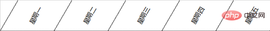
The first is: the tilt of the text (vertical text)

becomes

The actual operation is very simple, select the cells that need to be adjusted, right-click the mouse to bring up the "Format Cells" window - "Align" - click vertical "Text" under "Direction" - OK.
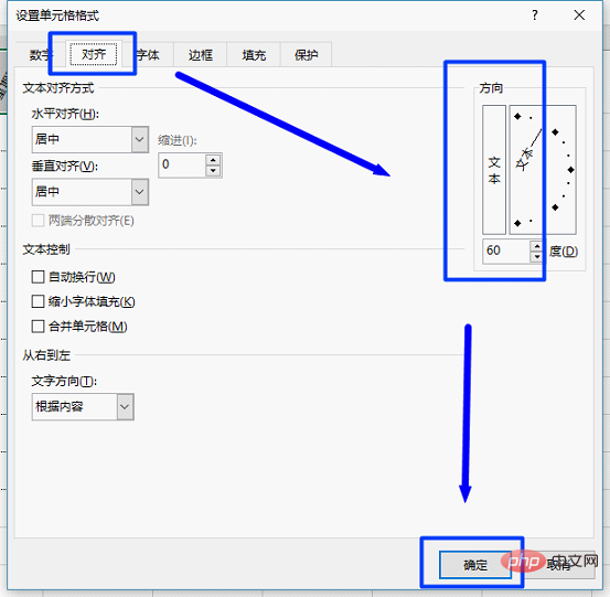
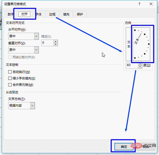
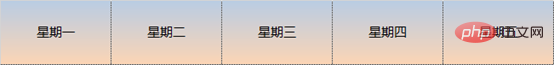
The second is: the tilt of the cell

becomes
It is also set in "Format Cells" - "Alignment" - "Direction". But this time, the angle on the right side is adjusted. You can drag it with the mouse or enter the angle value on the keyboard below.
4. Beautification of the header
In order to highlight the header, many people like to set it to a gradient color to make it clear at a glance.
becomes
Many donors only know how to set cells to one color, then how to change it to a gradient color Woolen cloth?
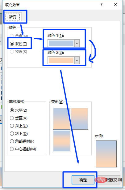
Right-click the mouse on the selected cell, set the cell format - fill - fill effect.
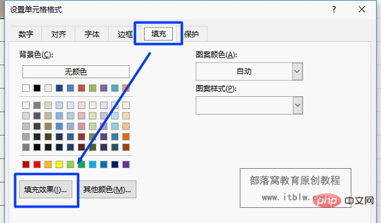
#You can set countless background colors according to the following picture.
5. Repeat header
The "repeat header" function is used in many scenarios. For example, the human resources department prints salary slips to employees every month. If you insert blank lines line by line - copy headers - paste headers, it will really affect work efficiency, and you have to do it again every month. Is there any What's a good idea?
In fact, there are many ways, you can use functions, you can use pivot tables, you can also set up your own "macro". Today, I will teach the donor the quick method that is best understood and learned fastest.
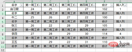
Step one: Insert a blank column at the end of the table and fill in a number sequence (1, 2, 3...). And copy the number column below the table.
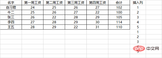
Step 2: Sort the "insert column" in ascending order. After the operation, you will find that there is an extra blank row in the middle of each person.
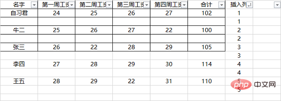
Step 3: After copying the header of the first row (note, copy first), select the first column and press F5 (or Ctrl G) to position - position condition.
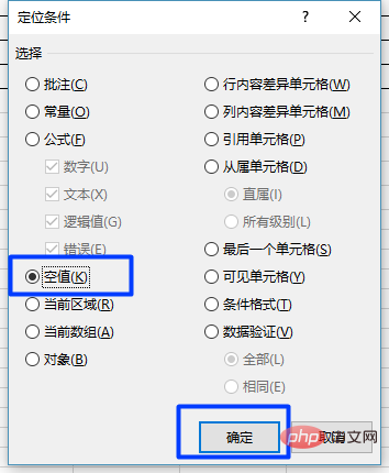
In the pop-up "Positioning Conditions" window, select "Null Value (K)" and confirm. All blank rows are selected.
Step 4: Direct shortcut key Ctrl V to paste.
6. Double row header combination display
Some excel table headers are very long, which is not conducive to our review and In contrast, excel has its own "combination" function, which is very convenient to use.

becomes
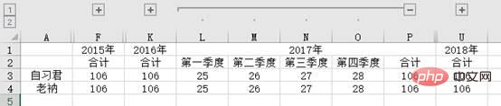
(Note: Click the " " and "-" signs in the above image to expand or summing up the four quarters of each year).
For the above functions, you only need to set the "combination" function in advance.
Step one: Select columns B:E, click "Data" - "Combination", and the year 2015 is set.
Step 2: Select columns B:F, click "Start" - "Format Painter", select columns G:U, and the "combination" function will be set up from 2016 to 2018.
If you want to cancel the hierarchical display, just click on the data - Ungroup.

7. The table header does not move when you scroll the mouse
Sometimes the Excel table is very long, and you scroll the mouse to see the numbers behind it, but the table header does not move. I forgot what the data represents, because the header has long since disappeared, and now I have to pull the scroll bar back and forth, which is very troublesome. In fact, Excel designers have already thought of these details, and only need to make one setting to solve this trouble.
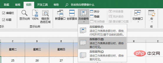
#Choose to freeze the first row: When scrolling the worksheet, the first row of the excel table remains unchanged.
Select Freeze First Column: When scrolling the worksheet, the first column of the excel table remains unchanged.
Click a cell and select Freeze Window: When scrolling the worksheet, all content above and to the left of this cell will remain motionless.
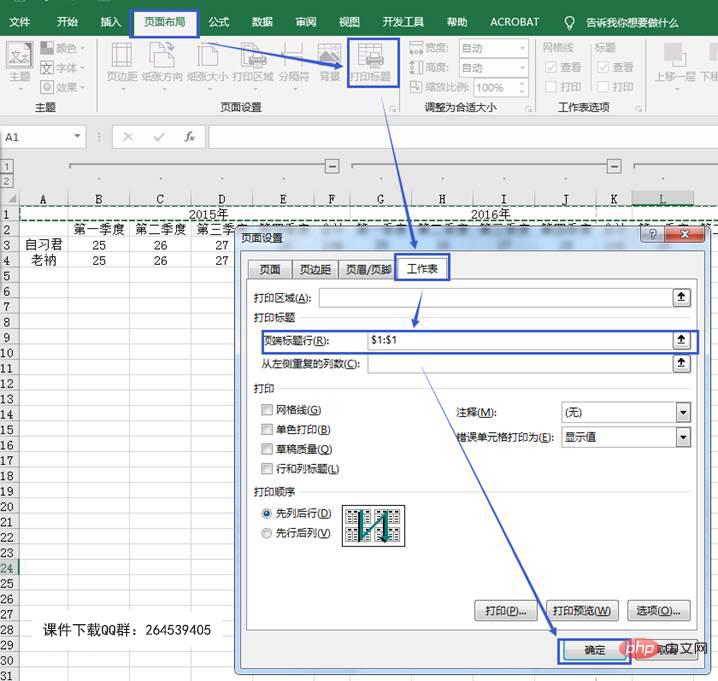
8. Each page has a header when printing
This function is very practical and often used.
Page layout - print title - worksheet - top title row, you can manually enter "$1:$1", or you can click the ↑ arrow on the right to select the title row, and finally click OK to see it in the print preview Let’s see the effect.
Related learning recommendations: excel tutorial
The above is the detailed content of Practical Excel skills sharing: 8 typical forms and problems of table headers. For more information, please follow other related articles on the PHP Chinese website!

Hot AI Tools

Undresser.AI Undress
AI-powered app for creating realistic nude photos

AI Clothes Remover
Online AI tool for removing clothes from photos.

Undress AI Tool
Undress images for free

Clothoff.io
AI clothes remover

Video Face Swap
Swap faces in any video effortlessly with our completely free AI face swap tool!

Hot Article
Hot Tools

Notepad++7.3.1
Easy-to-use and free code editor

SublimeText3 Chinese version
Chinese version, very easy to use

Zend Studio 13.0.1
Powerful PHP integrated development environment

Dreamweaver CS6
Visual web development tools

SublimeText3 Mac version
God-level code editing software (SublimeText3)
Hot Topics


 What should I do if the frame line disappears when printing in Excel?
Mar 21, 2024 am 09:50 AM
What should I do if the frame line disappears when printing in Excel?
Mar 21, 2024 am 09:50 AM
If when opening a file that needs to be printed, we will find that the table frame line has disappeared for some reason in the print preview. When encountering such a situation, we must deal with it in time. If this also appears in your print file If you have questions like this, then join the editor to learn the following course: What should I do if the frame line disappears when printing a table in Excel? 1. Open a file that needs to be printed, as shown in the figure below. 2. Select all required content areas, as shown in the figure below. 3. Right-click the mouse and select the "Format Cells" option, as shown in the figure below. 4. Click the “Border” option at the top of the window, as shown in the figure below. 5. Select the thin solid line pattern in the line style on the left, as shown in the figure below. 6. Select "Outer Border"
 How to filter more than 3 keywords at the same time in excel
Mar 21, 2024 pm 03:16 PM
How to filter more than 3 keywords at the same time in excel
Mar 21, 2024 pm 03:16 PM
Excel is often used to process data in daily office work, and it is often necessary to use the "filter" function. When we choose to perform "filtering" in Excel, we can only filter up to two conditions for the same column. So, do you know how to filter more than 3 keywords at the same time in Excel? Next, let me demonstrate it to you. The first method is to gradually add the conditions to the filter. If you want to filter out three qualifying details at the same time, you first need to filter out one of them step by step. At the beginning, you can first filter out employees with the surname "Wang" based on the conditions. Then click [OK], and then check [Add current selection to filter] in the filter results. The steps are as follows. Similarly, perform filtering separately again
 How to change excel table compatibility mode to normal mode
Mar 20, 2024 pm 08:01 PM
How to change excel table compatibility mode to normal mode
Mar 20, 2024 pm 08:01 PM
In our daily work and study, we copy Excel files from others, open them to add content or re-edit them, and then save them. Sometimes a compatibility check dialog box will appear, which is very troublesome. I don’t know Excel software. , can it be changed to normal mode? So below, the editor will bring you detailed steps to solve this problem, let us learn together. Finally, be sure to remember to save it. 1. Open a worksheet and display an additional compatibility mode in the name of the worksheet, as shown in the figure. 2. In this worksheet, after modifying the content and saving it, the dialog box of the compatibility checker always pops up. It is very troublesome to see this page, as shown in the figure. 3. Click the Office button, click Save As, and then
 How to type subscript in excel
Mar 20, 2024 am 11:31 AM
How to type subscript in excel
Mar 20, 2024 am 11:31 AM
eWe often use Excel to make some data tables and the like. Sometimes when entering parameter values, we need to superscript or subscript a certain number. For example, mathematical formulas are often used. So how do you type the subscript in Excel? ?Let’s take a look at the detailed steps: 1. Superscript method: 1. First, enter a3 (3 is superscript) in Excel. 2. Select the number "3", right-click and select "Format Cells". 3. Click "Superscript" and then "OK". 4. Look, the effect is like this. 2. Subscript method: 1. Similar to the superscript setting method, enter "ln310" (3 is the subscript) in the cell, select the number "3", right-click and select "Format Cells". 2. Check "Subscript" and click "OK"
 How to set superscript in excel
Mar 20, 2024 pm 04:30 PM
How to set superscript in excel
Mar 20, 2024 pm 04:30 PM
When processing data, sometimes we encounter data that contains various symbols such as multiples, temperatures, etc. Do you know how to set superscripts in Excel? When we use Excel to process data, if we do not set superscripts, it will make it more troublesome to enter a lot of our data. Today, the editor will bring you the specific setting method of excel superscript. 1. First, let us open the Microsoft Office Excel document on the desktop and select the text that needs to be modified into superscript, as shown in the figure. 2. Then, right-click and select the "Format Cells" option in the menu that appears after clicking, as shown in the figure. 3. Next, in the “Format Cells” dialog box that pops up automatically
 How to use the iif function in excel
Mar 20, 2024 pm 06:10 PM
How to use the iif function in excel
Mar 20, 2024 pm 06:10 PM
Most users use Excel to process table data. In fact, Excel also has a VBA program. Apart from experts, not many users have used this function. The iif function is often used when writing in VBA. It is actually the same as if The functions of the functions are similar. Let me introduce to you the usage of the iif function. There are iif functions in SQL statements and VBA code in Excel. The iif function is similar to the IF function in the excel worksheet. It performs true and false value judgment and returns different results based on the logically calculated true and false values. IF function usage is (condition, yes, no). IF statement and IIF function in VBA. The former IF statement is a control statement that can execute different statements according to conditions. The latter
 Where to set excel reading mode
Mar 21, 2024 am 08:40 AM
Where to set excel reading mode
Mar 21, 2024 am 08:40 AM
In the study of software, we are accustomed to using excel, not only because it is convenient, but also because it can meet a variety of formats needed in actual work, and excel is very flexible to use, and there is a mode that is convenient for reading. Today I brought For everyone: where to set the excel reading mode. 1. Turn on the computer, then open the Excel application and find the target data. 2. There are two ways to set the reading mode in Excel. The first one: In Excel, there are a large number of convenient processing methods distributed in the Excel layout. In the lower right corner of Excel, there is a shortcut to set the reading mode. Find the pattern of the cross mark and click it to enter the reading mode. There is a small three-dimensional mark on the right side of the cross mark.
 How to insert excel icons into PPT slides
Mar 26, 2024 pm 05:40 PM
How to insert excel icons into PPT slides
Mar 26, 2024 pm 05:40 PM
1. Open the PPT and turn the page to the page where you need to insert the excel icon. Click the Insert tab. 2. Click [Object]. 3. The following dialog box will pop up. 4. Click [Create from file] and click [Browse]. 5. Select the excel table to be inserted. 6. Click OK and the following page will pop up. 7. Check [Show as icon]. 8. Click OK.
