

How vlookup matches multiple columns of data


If we are given one column of data now, but we are asked to match multiple columns of data, how should we solve this problem?
The above questions are the examples we are going to explain today, so next we will directly enter the example explanation stage.
Example: We now have such an excel worksheet, which contains two tables. The first table is a data source table, which includes five items: customer ID, company name, contact name, address and contact title, along with related data. The second table contains four items, respectively. It is the customer ID, company name, contact name and address, where the customer ID is known content, while the company name, contact name and address are unknown content. Now our task is to based on the data source in the first table and the second table For the customer ID in the table, use the function vlookup to match the company name, contact name and address. The excel worksheet is as follows:

Example picture
Here, I recommend two methods to solve this problem.
Method 1: In H2 cell, I2 cell and J2 cell respectively, you can also use the function vlookup to get the corresponding results, and then use the drag function of the fill handle to get All cells to be matched.
The specific operation method is as follows: First, we enter "=VLOOKUP(G2,$A$1:$E$16,2,0)", "= in cell H2, cell I2 and cell J2 in sequence VLOOKUP(G2,$A$1:$E$16,3,0)", "=VLOOKUP(G2,$A$1:$E$16,4,0)", then we press the Enter key to get the customers respectively The company name, contact name and address corresponding to the ID "BERGS", then we select the H2 cell, I2 cell and J2 cell, and then drag down by dragging the fill handle, we can go to other The company name, contact name and address corresponding to the customer ID. For specific operations, please refer to the picture below:

Example picture
Method evaluation: The above method combines the basic usage of the function vlookup with the dragging function of the fill handle. It solves the existing problems, but it still has great limitations. Just imagine, here we have to match three items of data, and we end up writing three formulas. If we match 100 items of data, I'm afraid we don't have the patience to write another 100 formulas. So let’s look at the more convenient method two next!
Method 2: Here we only need to fill in the appropriate function formula in the H2 cell, and then use the fill handle to drag left and down, so that all results can be obtained . But in this process we will encounter two major problems: How to make mixed references to the first parameter? How to determine the third parameter? Next, we will solve the problem while making a table.
First, we make the answer to cell H2. Enter "=VLOOKUP(G2,$A$1:$E$16,2,0)" in cell H2 and press Enter. At this time, based on past experience, we know that if we drag down next, the result will still not be wrong, so the key question is how to ensure that dragging to the left will not go wrong.
We select cell H2 and drag one cell to the left to see what the result is?

Example picture
The result is #NA, the specific function formula is "=VLOOKUP(H2,$A$1:$E$16,2,0) ", from this functional formula, we can see two errors. First, the first parameter should be "G2", not "H2", and secondly, the third parameter should be "3", not "2".
First of all, let’s solve the problem caused by the first parameter. Some people may say that it can be changed to $G$2 (absolute reference). This does solve the problem caused by dragging to the left, but it also It will cause an error when dragging down, so we need to use mixed references to solve the problem. Rewrite "G2" to "$G2" and lock the column.
Now we come to the second question, how to make the third parameter change continuously as the fill handle is dragged? We can see from the functional formula "=VLOOKUP(H2,$A$1:$E$16,2,0)" that if you just fill in the numbers in the function vlookup, it will not continue to change as the fill handle is dragged. , so we still need to use the functions of functions.
excel
Here I recommend using the function column. Its basic grammatical form is COLUMN(reference). Specifically, we can look at the following three examples: "=COLUMN()" will get the formula. column; "=COLUMN(A10)" will get the result "1" because column A is the first column; "=COLUMN(C3:D10)" will get the column number of the first column in the reference, which is "3". What we want to use here is "=COLUMN()".
Here when we enter "=COLUMN()" in cell H2, we will get "8", because column H is the eighth column, but the third parameter here should be "2", so the specific value of the third parameter The format should be "=COLUMN()-6". At this time, the functional formula to be filled in cell H2 will become "=VLOOKUP($G2,$A$1:$E$16,COLUMN()-6,0)" ". When dragging to the left, the first parameter G2 remains unchanged, and the third parameter "COLUMN()-6" increases accordingly; when dragging downward, the first parameter changes accordingly, and the third parameter "COLUMN() )-6" remains unchanged, such a functional expression meets all requirements.
Specific method arrangement: First, we enter "=VLOOKUP($G2,$A$1:$E$16,COLUMN()-6,0)" in cell H2, and then we press the Enter key. We can get the company name corresponding to the customer ID "BERGS" respectively. Then we select the H2 cell and drag it to the left to get the contact name and address corresponding to the customer ID "BERGS". Finally, we select cell H2, cell I2 and cell J2, and then drag down by dragging the fill handle. We can get the company name, contact name and address corresponding to other customer IDs. For specific operations, please refer to the picture below:

Example picture
Summary:
1. First of all, we must be very proficient in using the function vlookup For basic operation methods, if you are interested, you can refer to the article Thousands of data are fascinating, and the function vlookup will help you choose!
2. The issues of relative reference, absolute reference and mixed reference of cell content in excel must be clearly distinguished. You can refer to the article Excel about the clever use of absolute reference and mixed reference.
3. To understand Understand the basic usage of function column.
Today’s sharing ends here, interested friends can like and follow!
For more technical articles related to frequently asked questions, please visit the FAQ column to learn more!
The above is the detailed content of How vlookup matches multiple columns of data. For more information, please follow other related articles on the PHP Chinese website!

Hot AI Tools

Undresser.AI Undress
AI-powered app for creating realistic nude photos

AI Clothes Remover
Online AI tool for removing clothes from photos.

Undress AI Tool
Undress images for free

Clothoff.io
AI clothes remover

Video Face Swap
Swap faces in any video effortlessly with our completely free AI face swap tool!

Hot Article
Hot Tools

Notepad++7.3.1
Easy-to-use and free code editor

SublimeText3 Chinese version
Chinese version, very easy to use

Zend Studio 13.0.1
Powerful PHP integrated development environment

Dreamweaver CS6
Visual web development tools

SublimeText3 Mac version
God-level code editing software (SublimeText3)
Hot Topics


 Parameters of vlookup function and explanation of their meanings
Jan 09, 2024 pm 03:18 PM
Parameters of vlookup function and explanation of their meanings
Jan 09, 2024 pm 03:18 PM
We must have used the vlookup function when using excel. So there are several such functions, and how each function is used. As far as the editor knows, there are four vlookup functions, namely Lookup_value, Table_array, col_index_num, and Range_lookup. So let me tell you their specific usage~ The vlookup function has several parameters and the meaning of each parameter. The parameters of the vlookup function include Lookup_value, Table_array, col_index_num, and Range_lookup, a total of 4. 1.Lookup
 How to use vlookup function to match across tables
Feb 20, 2024 pm 11:30 PM
How to use vlookup function to match across tables
Feb 20, 2024 pm 11:30 PM
The vlookup function is one of the most commonly used functions in Excel. It can help us find a specified value in a table and return the corresponding value in another table that matches the value. In this article, we will explore the use of the vlookup function, especially when performing cross-table matching. First, let's learn the basic syntax of the vlookup function. In Excel, the syntax of the vlookup function is as follows: =vlookup(lookup_value,ta
 An error occurred when using the vlookup function
Feb 21, 2024 pm 12:18 PM
An error occurred when using the vlookup function
Feb 21, 2024 pm 12:18 PM
The vlookup function is a very commonly used search function in Excel. It is used to find a value in a specified data range and return its corresponding data. However, many people may encounter some errors when using the vlookup function. This article will introduce some common vlookup function usage errors and provide solutions. Before using the vlookup function, you first need to understand its syntax. The syntax of the vlookup function is as follows: =VLOOKUP(lookup_value,ta
 How to use the vlookup function-How to use the vlookup function
Mar 04, 2024 pm 12:31 PM
How to use the vlookup function-How to use the vlookup function
Mar 04, 2024 pm 12:31 PM
Many friends don't know how to use the vlookup function, so the editor will share how to use the vlookup function below. Let's take a look. I believe it will be helpful to everyone. 1. Accurate search According to the accurate information, query the corresponding data in the data table. In the figure, you can search the student ID by name and use "=VLOOKUP(F3,A1:D5,4,0)". 2. Multi-condition search If there are duplicate data in the table, you need to add conditions to limit the query. The formula used to find Class 2 Li Bai in the picture is "=VLOOKUP(F5&G5,IF({1,0},A3:A11&B3:B11,D3:D11),2,FALSE)". 3. For reverse lookup, we want to use VLOOK
 How to use formula vlookup
Feb 19, 2024 pm 10:37 PM
How to use formula vlookup
Feb 19, 2024 pm 10:37 PM
The formula VLOOKUP is a very commonly used function in Microsoft Excel. It is used to find a specific value in a table or data set and return other values associated with it. In this article, we will learn how to use the VLOOKUP formula correctly. The basic syntax of the VLOOKUP function is as follows: VLOOKUP(lookup_value, table_array, col_index_num, [range_lookup]) where: lookup
 Application of VLOOKUP function in Excel function formula
Mar 20, 2024 am 11:30 AM
Application of VLOOKUP function in Excel function formula
Mar 20, 2024 am 11:30 AM
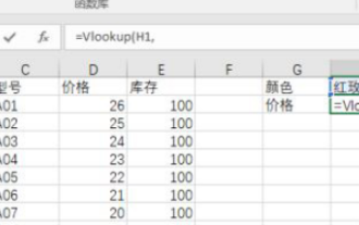
There are many function formulas, but not all of them are easy to use. In the past, I preferred to use index and match to achieve what Vlookup can do. But after I really got to know the Vlookup family, I decided to use index and match. Instead of using the Vlookup function, I will now introduce the Vlookup function formula to the readers in detail. First we need to enter the formula =Vlookup(H1, conditional area, return the number of area columns, precise or approximate), where H1 is the position of the red rose. After that, we will add the formula. How to choose this conditional area? This area requires the condition to be in the first column, which is the column with the color of our red rose. It must be this
 Steps to use the VLOOKUP function
Feb 19, 2024 pm 03:54 PM
Steps to use the VLOOKUP function
Feb 19, 2024 pm 03:54 PM
The vlookup function is a very commonly used function in Excel and plays an important role in data processing and analysis. It can search for matching values in a data table based on specified keywords and return corresponding results, providing users with the ability to quickly find and match data. The following will introduce the use of the vlookup function in detail. The basic syntax of the vlookup function is: =VLOOKUP(lookup_value,table_array,col_index
 How to use the VLOOKUP function
Feb 18, 2024 pm 06:41 PM
How to use the VLOOKUP function
Feb 18, 2024 pm 06:41 PM
vlookup is a very useful function in Excel. It can find relevant data in a column or table based on specified conditions and return the results. When processing large amounts of data or needing to perform data matching, vlookup can greatly improve work efficiency. To use the vlookup function, you first need to determine the range of the data you want to find and the conditions you want to match. The syntax of vlookup is as follows: vlookup (value to be found, range, index of the returned column, whether it matches exactly
