

INDEX MATCH MATCH in Excel for two-dimensional lookup

The tutorial showcases a few different formulas to perform two dimensional lookup in Excel. Just look through the alternatives and choose your favorite :)
When searching for something in your Excel spreadsheets, most of the time you'd look up vertically in columns or horizontally in rows. But sometimes you need to look across both rows and columns. In other words, you aim to find a value at the intersection of a certain row and column. This is called matrix lookup (aka 2-dimensional or 2-way lookup), and this tutorial shows how to do it in 4 different ways.
Excel INDEX MATCH MATCH formula
The most popular way to do a two-way lookup in Excel is by using INDEX MATCH MATCH. This is a variation of the classic INDEX MATCH formula to which you add one more MATCH function in order to get both the row and column numbers:
INDEX (data_array, MATCH (vlookup_value, lookup_column_range, 0), MATCH (hlookup value, lookup_row_range, 0))As an example, let's make a formula to pull a population of a certain animal in a given year from the table below. For starters, we define all the arguments:
- Data_array - B2:E4 (data cells, not including row and column headers)
- Vlookup_value - H1 (target animal)
- Lookup_column_range - A2:A4 (row headers: animal names) - A3:A4
- Hlookup_value - H2 (target year)
- Lookup_row_range - B1:E1 (column headers: years)
Put all the arguments together and you will get this formula for two-way lookup:
=INDEX(B2:E4, MATCH(H1, A2:A4, 0), MATCH(H2, B1:E1, 0))

If you need to do a two-way lookup with more than two criteria, take a look at this article: INDEX MATCH with multiple criteria in rows and columns.
How this formula works
While it may look a bit complex at first glance, the formula's logic is really straightforward and easy to understand. The INDEX function retrieves a value from the data array based on the row and column numbers, and two MATCH functions supply those numbers:
INDEX(B2:E4, row_num, column_num)
Here, we leverage the ability of MATCH(lookup_value, lookup_array, [match_type]) to return a relative position of lookup_value in lookup_array.
So, to get the row number, we search for the animal of interest (H1) across the row headers (A2:A4):
MATCH(H1, A2:A4, 0)
To get the column number, we search for the target year (H2) across the column headers (B1:E1):
MATCH(H2, B1:E1, 0)
In both cases, we look for exact match by setting the 3rd argument to 0.
In this example, the first MATCH returns 2 because our vlookup value (Polar bear) is found in A3, which is the 2nd cell in A2:A4. The second MATCH returns 3 because the hlookup value (2000) is found in D1, which is the 3rd cell in B1:E1.
Given the above, the formula reduces to:
INDEX(B2:E4, 2, 3)
And return a value at the intersection of the 2nd row and 3rd column in the data array B2:E4, which is a value in the cell D3.
VLOOKUP and MATCH formula for 2-way lookup
Another way to do a two-dimensional lookup in Excel is by using a combination of VLOOKUP and MATCH functions:
VLOOKUP(vlookup_value, table_array, MATCH(hlookup_value, lookup_row_range, 0), FALSE)For our sample table, the formula takes the following shape:
=VLOOKUP(H1, A2:E4, MATCH(H2, A1:E1, 0), FALSE)
Where:
- Table_array - A2:E4 (data cells including row headers)
- Vlookup_value - H1 (target animal)
- Hlookup_value - H2 (target year)
- Lookup_row_range - A1:E1 (column headers: years)

How this formula works
The core of the formula is the VLOOKUP function configured for exact match (the last argument set to FALSE), which searches for the lookup value (H1) in the first column of the table array (A2:E4) and returns a value from another column in the same row. To determine which column to return a value from, you use the MATCH function that is also configured for exact match (the last argument set to 0):
MATCH(H2, A1:E1, 0)
MATCH searches for the value in H2 across the column headers (A1:E1) and returns the relative position of the found cell. In our case, the target year (2010) is found in E1, which is 5th in the lookup array. So, the number 5 goes to the col_index_num argument of VLOOKUP:
VLOOKUP(H1, A2:E4, 5, FALSE)
VLOOKUP takes it from there, finds an exact match for its lookup value in A2 and returns a value from the 5th column in the same row, which is the cell E2.
Important note! For the formula to work correctly, table_array (A2:E4) of VLOOKUP and lookup_array of MATCH (A1:E1) must have the same number of columns, otherwise the number passed by MATCH to col_index_num will be incorrect (won't correspond to the column's position in table_array).
XLOOKUP function to look in rows and columns
Recently Microsoft has introduced one more function in Excel that is meant to replace all existing lookup functions such as VLOOKUP, HLOOKUP and INDEX MATCH. Among other things, XLOOKUP can look at the intersection of a specific row and column:
XLOOKUP(vlookup_value, vlookup_column_range, XLOOKUP(hlookup_value, hlookup_row_range, data_array))For our sample data set, the formula goes as follows:
=XLOOKUP(H1, A2:A4, XLOOKUP(H2, B1:E1, B2:E4))

Note. The XLOOKUP function is only available in Excel for Microsoft 365, Excel 2021, and Excel for the web.
How this formula works
The formula uses the ability of XLOOKUP to return an entire row or column. The inner function searches for the target year in the header row and returns all the values for that year (in this example, for year 1980). Those values go to the return_array argument of the outer XLOOKUP:
XLOOKUP(H1, A2:A4, {22000;25000;700}))
The outer XLOOKUP function searches for the target animal across the column headers and returns the value in the same position from the return_array.
SUMPRODUCT formula for two-way lookup
The SUMPRODUCT function is like a Swiss knife in Excel – it can do so many things beyond its designated purpose, especially when it comes to evaluating multiple criteria.
To look up two criteria, in rows and columns, use this generic formula:
SUMPRODUCT(vlookup_column_range = vlookup_value) * (hlookup_row_range = hlookup_value), data_array)To perform a 2-way lookup in our dataset, the formula goes as follows:
=SUMPRODUCT((A2:A4=H1) * (B1:E1=H2), B2:E4)
The below syntax will work too:
=SUMPRODUCT((A2:A4=H1) * (B1:E1=H2) * B2:E4)

How this formula works
At the heart of the formula, we compare two lookup values against the row and column headers (the target animal in H1 against all animal names in A2:A4 and the target year in H2 against all years in B1:E1):
(A2:A4=H1) * (B1:E1=H2)
This results in 2 arrays of TRUE and FALSE values, where TRUE's represent matches:
{FALSE;FALSE;TRUE} * {FALSE,TRUE,FALSE,FALSE}
The multiplication operation coerces the TRUE and FALSE values into 1's and 0's and produces a two-dimensional array of 4 columns and 3 rows (rows are separated by semicolons and each column of data by a comma):
{0,0,0,0;0,0,0,0;0,1,0,0}
The SUMPRODUCT functions multiplies the elements of the above array by the items of B2:E4 in the same positions:
{0,0,0,0;0,0,0,0;0,1,0,0} * {22000,13800,8500,3500;25000,23000,22000,20000;700,2000,2300,2500}
And because multiplying by zero gives zero, only the item corresponding to 1 in the first array survives:
SUMPRODUCT({0,0,0,0;0,0,0,0;0,2000,0,0})
Finally, SUMPRODUCT adds up the elements of the resulting array and returns a value of 2000.
Note. If your table has more than one row or/and column headers with the same name, the final array will contain more than one number other than zero, and all those numbers will be added up. As the result, you will get a sum of values that meet both criteria. It is what makes the SUMPRODUCT formula different from INDEX MATCH MATCH and VLOOKUP, which return the first found match.
Matrix lookup with named ranges (explicit Intersection)
One more amazingly simple way to do a matrix lookup in Excel is by using named ranges. Here's how:
Part 1: Name columns and rows
The fastest way to name each row and each column in your table is this:
- Select the whole table (A1:E4 in our case).
- On the Formulas tab, in the Defined Names group, click Create from Selection or press the Ctrl Shift F3 shortcut.
- In the Create Names from Selection dialog box, select Top row and Left column, and click OK.


This automatically creates names based on the row and column headers. However, there are a couple of caveats:
- If your column and/or rows headers are numbers or contain specific characters that are not allowed in Excel names, the names for such columns and rows won't be created. To see a list of created names, open the Name Manager (Ctrl F3). If some names are missing, define them manually as explained in How to name a range in Excel.
- If some of your row or column headers contain spaces, the spaces will be replaced with underscores, for example, Polar_bear.
For our sample table, Excel automatically created only the row names. The column names have to be created manually because the column headers are numbers. To overcome this, you can simply preface the numbers with underscores, like _1990.
As the result, we have the following named ranges:

Part 2: Make a matrix lookup formula
To pull a value at the intersection of a given row and column, just type one of the following generic formulas in an empty cell:
=row_name column_nameOr vice versa:
=column_name row_nameFor example, to get the population of blue whales in 1990, the formula is as simple as:
=Blue_whale _1990
If someone needs more detailed instructions, the following steps will walk you through the process:
- In a cell where you want the result to appear, type the equality sign (=).
- Start typing the name of the target row, say, Blue_whale. After you've typed a couple of characters, Excel will display all existing names that match your input. Double-click the desired name to enter it in your formula:
- After the row name, type a space, which works as the intersection operator in this case.
- Enter the target column name ( _1990 in our case).
- As soon as both the row and column names are entered, Excel will highlight the corresponding row and column in your table, and you press Enter to complete the formula:


Your matrix lookup is done, and the below screenshot shows the result:

That's how to look up in rows and columns in Excel. I thank you for reading and hope to see you on our blog next week!
Available downloads
2-dimensional lookup sample workbook
The above is the detailed content of INDEX MATCH MATCH in Excel for two-dimensional lookup. For more information, please follow other related articles on the PHP Chinese website!

Hot AI Tools

Undresser.AI Undress
AI-powered app for creating realistic nude photos

AI Clothes Remover
Online AI tool for removing clothes from photos.

Undress AI Tool
Undress images for free

Clothoff.io
AI clothes remover

Video Face Swap
Swap faces in any video effortlessly with our completely free AI face swap tool!

Hot Article
Hot Tools

Notepad++7.3.1
Easy-to-use and free code editor

SublimeText3 Chinese version
Chinese version, very easy to use

Zend Studio 13.0.1
Powerful PHP integrated development environment

Dreamweaver CS6
Visual web development tools

SublimeText3 Mac version
God-level code editing software (SublimeText3)
Hot Topics


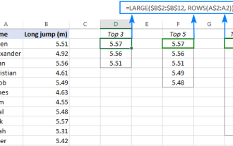 Excel formula to find top 3, 5, 10 values in column or row
Apr 01, 2025 am 05:09 AM
Excel formula to find top 3, 5, 10 values in column or row
Apr 01, 2025 am 05:09 AM
This tutorial demonstrates how to efficiently locate the top N values within a dataset and retrieve associated data using Excel formulas. Whether you need the highest, lowest, or those meeting specific criteria, this guide provides solutions. Findi
 Add a dropdown list to Outlook email template
Apr 01, 2025 am 05:13 AM
Add a dropdown list to Outlook email template
Apr 01, 2025 am 05:13 AM
This tutorial shows you how to add dropdown lists to your Outlook email templates, including multiple selections and database population. While Outlook doesn't directly support dropdowns, this guide provides creative workarounds. Email templates sav
 How to use Flash Fill in Excel with examples
Apr 05, 2025 am 09:15 AM
How to use Flash Fill in Excel with examples
Apr 05, 2025 am 09:15 AM
This tutorial provides a comprehensive guide to Excel's Flash Fill feature, a powerful tool for automating data entry tasks. It covers various aspects, from its definition and location to advanced usage and troubleshooting. Understanding Excel's Fla
 How to add calendar to Outlook: shared, Internet calendar, iCal file
Apr 03, 2025 am 09:06 AM
How to add calendar to Outlook: shared, Internet calendar, iCal file
Apr 03, 2025 am 09:06 AM
This article explains how to access and utilize shared calendars within the Outlook desktop application, including importing iCalendar files. Previously, we covered sharing your Outlook calendar. Now, let's explore how to view calendars shared with
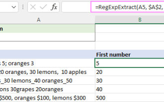 Regex to extract strings in Excel (one or all matches)
Mar 28, 2025 pm 12:19 PM
Regex to extract strings in Excel (one or all matches)
Mar 28, 2025 pm 12:19 PM
In this tutorial, you'll learn how to use regular expressions in Excel to find and extract substrings matching a given pattern. Microsoft Excel provides a number of functions to extract text from cells. Those functions can cope with most
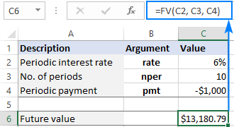 FV function in Excel to calculate future value
Apr 01, 2025 am 04:57 AM
FV function in Excel to calculate future value
Apr 01, 2025 am 04:57 AM
This tutorial explains how to use Excel's FV function to determine the future value of investments, encompassing both regular payments and lump-sum deposits. Effective financial planning hinges on understanding investment growth, and this guide prov
 MEDIAN formula in Excel - practical examples
Apr 11, 2025 pm 12:08 PM
MEDIAN formula in Excel - practical examples
Apr 11, 2025 pm 12:08 PM
This tutorial explains how to calculate the median of numerical data in Excel using the MEDIAN function. The median, a key measure of central tendency, identifies the middle value in a dataset, offering a more robust representation of central tenden
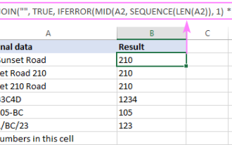 How to remove / split text and numbers in Excel cell
Apr 01, 2025 am 05:07 AM
How to remove / split text and numbers in Excel cell
Apr 01, 2025 am 05:07 AM
This tutorial demonstrates several methods for separating text and numbers within Excel cells, utilizing both built-in functions and custom VBA functions. You'll learn how to extract numbers while removing text, isolate text while discarding numbers
