Auto-format Excel GROUPBY and PIVOTBY results with conditional formatting

Learn how to turn your data into clear and colorful summary reports using Excel's GROUPBY and PIVOTBY formulas, enhanced with conditional formatting.

You have probably heard about the two recent additions to Excel's dynamic array functions: GROUPBY and PIVOTBY. These functions excel at grouping and summarizing data, but the results often appear plain and difficult to comprehend due to a lack of formatting. For better readability and presentation, you can, of course, manually format the key elements, such as headers, subtotals and totals. However, since the resulting array is dynamic, these elements may move around to accommodate changes in the original dataset. Naturally, you wouldn't want to reformat the data each time it changes. Fortunately, you can automate this process with conditional formatting, which updates dynamically based on the criteria you set.

• How to use conditional formatting with GROUPBY and PIVOTBY formulas
• Conditionally format GROUPBY results
• Conditionally format PIVOTBY results

How to apply conditional formatting to GROUPBY and PIVOTBY results

To format the results of your GROUPBY or PIVOTBY formulas automatically, you'll need to set up several conditional formatting rules based on formulas. The steps are universal for all rules, whether you're highlighting headers, subtotals, or totals. The variation lies in a particular formula used to identify each element and the formatting details. Please follow these recommendations closely to ensure optimal results:

1. Select the range to format. Begin by selecting all the results returned by your GROUPBY or PIVOTBY formula. If your original dataset is subject to change and you anticipate future additions, extend your selection to include additional blank rows below. This way, when more data is added, the conditional formatting will apply automatically.
2. Access Conditional Formatting. On the Home tab, click Conditional Formatting > New Rule…
3. Create a formula-based rule. In the New Formatting Rule window, select Use a formula to determine which cells to format. Then, enter the formula in the corresponding box.
4. Choose formats. Hit the Format button to open the formatting options. Here, you can select the desired formats that will be applied based on your rule.
5. Save the rule. Confirm your settings by clicking OK as many times as required, which will save and apply your new conditional formatting rule.

For detailed instructions, see How to set Excel conditional formatting rule with formula.

Excel GROUPBY formula with conditional formatting

This example shows how to make the output of the GROUPBY function more readable by highlighting the main elements, such as the header row, subtotals and totals.

Select the applied range for conditional formatting

In this example, the GROUPBY formula returns a dynamic array spanning from F3 to H16. However, for our conditional formatting rules, we select the range F3 to H32. This includes extra blank rows to accommodate any future data additions, ensuring that the formatting automatically applies as new data is added to the source table.

With an appropriate range selected, click Conditional Formatting > New Rule… to set up the first rule.

Now, let's see exactly what formulas and formatting options we can use.

Format the header row

Formatting the header row of your GROUPBY results is vital for distinguishing it from the rest of your data.

To identify the header row, you can use a formula that searches for a specific word or phrase unique to the headings, which doesn't appear elsewhere in the dataset. Here are two approaches:

Exact match formula

Use this method if your headers contain unique consistent terms. For example, if "Project type" is the first header in the returned array, you can identify it by looking for the text "Project type" in column F:

=$F3="Project type"

Partial match formula

If your header might vary (e.g. "project type" or "project name"), use the SEARCH function for a partial match:

=SEARCH("project", $F3)

As the SEARCH function is case-insensitive, you can type your text in any letter case.

Note. Whichever formula you opt for, remember to use a mixed cell reference (like $F3). This locks the column and allows the row number to adjust, ensuring the formatting is applied consistently across the entire row.

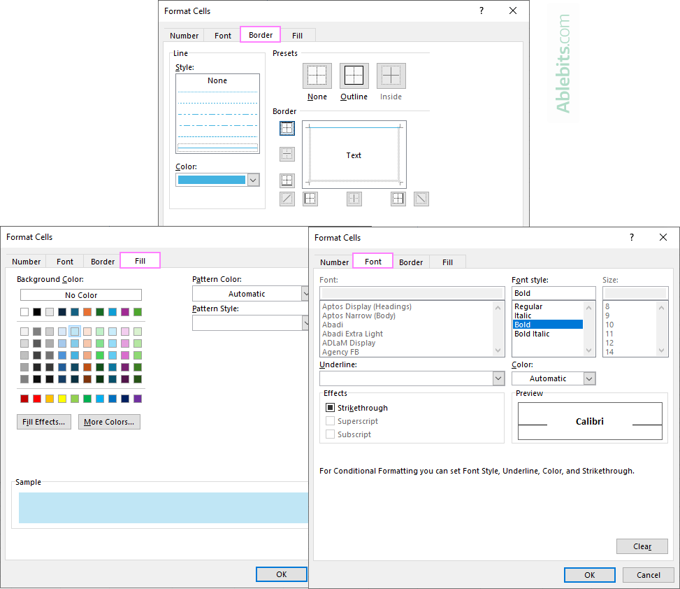
Formatting

Once you've set up your formula, proceed to apply bold formatting to the headers. In the Format Cells dialog box, go to the Font tab, and select Bold under Font Styles.

Additionally, you may want to add a colored line below the header row. For this, go to the Border tab, where you choose the desired line style and color and apply it to the lower cell border.

This simple yet effective formatting choice greatly improves the readability and professional appearance of your GROUPBY results.

Highlight subtotals

Enhancing the visibility of subtotals within the GROUPBY results can make your data analysis more intuitive and accessible. To achieve this, you'll need to accurately identify the subtotal rows. Typically, these rows contain values in the first-level grouping column (Project type in this example) and the aggregated columns (such as Revenue), while the cells in the secondary grouping column (such as Status) are empty.

Formula

To construct an appropriate formula, you can utilize the AND function that checks both conditions – whether column F (Project type) is not blank and column G (Status) is blank:

=AND($F3"", $G3="")

Be aware that the above formula will also format the grand total row since it meets both conditions. To refine the formula for highlighting subtotals while excluding the grand total, you can add one more logical test:

=AND($F3"", $G3="", $F3"grand total")

Formatting

To apply a background color to these identified rows, go to the Fill tab in the Format Cells dialog box. From there, you can select your preferred color, which will be applied to the subtotal rows.

Optionally, you can also format subtotals text in bold italic by choosing this option on the Font tab.

Format the grand total row

Bringing attention to the grand total is crucial for making the key summary of your data immediately noticeable.

Formula

To identify the grand total row, make a formula similar to the one used for the header row, but this time you search for the text "grand total." The formula is case-insensitive, so you can type the text in any case:

=$F3="grand total"

In Excel conditional formatting, cell references are relative to the top-left cell in the applied range. Therefore, we again write a formula for cell $F3 using a mixed reference – absolute column and relative row.

Formatting

To better distinguish the grand total row, we're going to change two elements - font and cell border:

• To emphasize the grand total text, navigate to the Font tab and select Bold under Font Styles.
• To add a line above the grand total row, switch to the Border tab. Here, select your preferred line style and color, and then apply the upper border to create a clear separation from the rest of the data.

Conditionally formatted GROUPBY results

The results of the GROUPBY formula, enhanced with conditional formatting, are not just well-organized but also aesthetically pleasing and intuitive to navigate.

Note. When formatting the GROUPBY output in your worksheets, remember to correctly adjust the references in conditional formatting formulas to match the layout of your specific dataset. For more information, see Cell references in Excel conditional formatting.

Excel PIVOTBY formula with conditional formatting

As you know, Excel PivotTables are automatically formatted to highlight headers, totals, and subtotals. For this example, we've created a PIVOTBY formula and PivotTable that group and aggregate the source data in the same way. And now, we will try to replicate the pivot table's format using conditional formatting to achieve a similar look for the PIVOTBY formula output.

Before creating a conditional formatting rule, select the results of your PIVOTBY formula. Optionally, include a few blank cells below to automatically format any new data that might be added later. In our case, we select the range G3:M32, and then click Conditional Formatting > New Rule… to start creating a rule for the header row.

Highlight the header row

The first step is to make the header row stand out.

Formula

In the dynamic array returned by the PIVOTBY formula, the first two cells in the header row are blank. You can check these two conditions using the following formula:

=AND($G3="", $H3="")

For the formatting to apply correctly to the entire row, remember to lock the columns and allow the row numbers to adjust by using mixed cell references like $G3 and $H3.

Formatting

For the headers to visually pop, consider applying three different formatting elements:

• Format text in bold. This makes the header text prominent.
• Add a line below. Format the lower cell border with a selected color to create a clear separation.
• Highlight. Set a fill color for the header row to make it visually distinct.

Highlight subtotals

If your PIVOTBY formula is configured to show subtotals, it makes sense to format them for better visibility and organization.

Formula

The formula to identify subtotal rows checks if a cell in column G is not blank and a cell in column H is blank. Additionally, it ensures it's not the grand total row, which is supposed to be formatted differently.

=AND($G3"", $H3="", $G3"grand total")

Formatting

For the formatting of subtotals, you can apply a combination of styles:

• Bold text. Apply bold formatting to the subtotal text to make it more visible.
• Line below. Add a line below the subtotal row to visually separate it from the data that follows.

Format the grand total row

The grand total row is the key summary of your data, so it should be prominently highlighted for quick reference.

Formula

To identify the grand total row, just check if a cell contains exactly this text:

=$G3="grand total"

Notice that the formula references the top-left cell in the applied range, even though the grand total is in the last row in the return array.

Formatting

To emphasize the grand total row, apply the following formatting:

• Bold text. Make the grand total text bold to highlight its importance.
• Line above. Add a line above the grand total row to separate it from the data above.
• Background color. Apply a distinct fill color to the grand total row to make it stand out.

Conditionally formatted PIVOTBY results

With the application of conditional formatting, the output of your PIVOTBY formula becomes visually comparable to a PivotTable, making it really nice and informative.

As we wrap up our article, I hope you feel ready to use these conditional formatting techniques to make your GROUPBY and PIVOTBY formulas tell a compelling story and look amazing.

Practice workbook for download

GROUPBY and PIVOTBY with conditional formatting (.xlsx file)

The above is the detailed content of Auto-format Excel GROUPBY and PIVOTBY results with conditional formatting. For more information, please follow other related articles on the PHP Chinese website!