Practical Excel skills sharing: data comparison in several different situations

Daily work requires comparing data, finding differences, finding duplicate values, etc. from time to time. Some compare data in the same worksheet, and some compare data between different worksheets. Here we summarize data comparisons in a variety of different situations, and provide quick methods so that everyone can quickly complete data comparisons under different situations.

Part 1: Comparison of data in the same table

1. Strict Compare whether the data in two columns are the same

# The so-called strict comparison refers to the comparison of data according to position.

1) Shortcut key comparison Ctrl

As shown in the figure below, select the two columns of data to be compared, column A and column B, and then press the shortcut key Ctrl. Different The data B5, B9, B10, and B15 will be selected.

2) Comparison of positioning methods (shortcut key F5 or Ctrl G)

The following table is an example, select columns A and Quickly select two columns of data in the column header of column B, then press the shortcut key F5 (or Ctrl G) to bring up the positioning window, select the positioning condition as "row content difference cells", click the "OK" button, different data will be selected.

Note:

The above two methods can quickly compare the differences between two columns of data, but they will not distinguish between uppercase and lowercase letters.

3) Comparison of IF functions

(1) Comparison of if functions that do not require case-sensitive letters

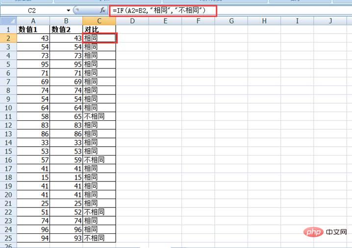
Both columns A and B in the table below are It is a number, there are no letters, and it does not need to be case sensitive.

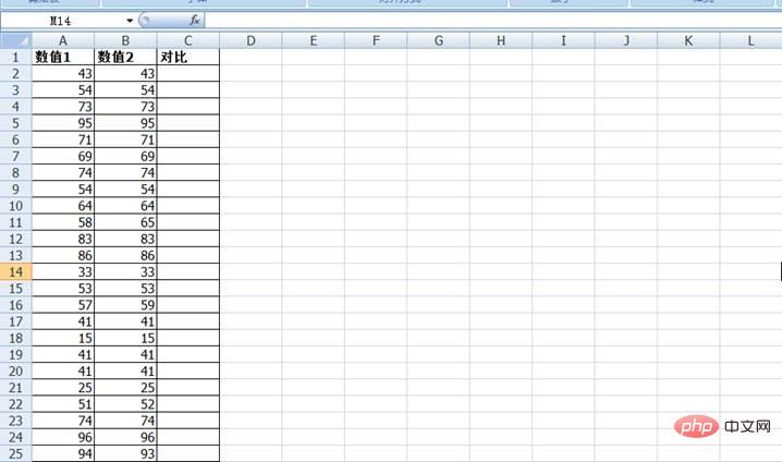
You can enter the formula =IF(A2=B2, "Same", "Not the same") in cell C2. After inputting, pull the handle and drag it down until The data in this column are cut off, and the same and different results are clear at a glance, as shown in the table below.

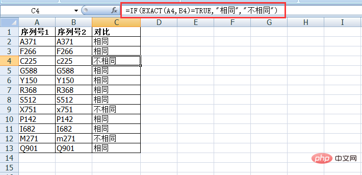
(2) Case-sensitive if function comparison

If the comparison data contains letters and needs to be case-sensitive, the above formula cannot be accurate Compared. At this time, you can change the C2 formula to =IF(EXACT(A2,B2)=TRUE,"Same","Not the same"), and then drop down to fill in the formula, as shown in the figure below.

2. Find duplicate values ​​in two columns of data

1) IF MATCH Function to find duplicate values

Now we want to find out the list of winners for two consecutive quarters in the following table, what method is there?

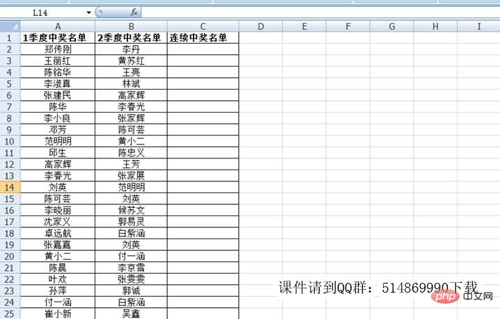
In fact, it is necessary to find duplicate values ​​by comparing column A and column B. We can use the IF MATCH function to combine formulas, enter the formula =IF(ISERROR(MATCH(A2,$B$2:$B$25,0)),"",A2) in cell C2, and then pull down Copy the formula to complete the search task. See the table below for comparison search results:

Formula analysis:

MATCH is used to return the position of the data A2 to be found in the area $B$2:$B$25. If it is found, a line number will be returned (indicating that there is a duplication), if not found, an error #N/A will be returned (indicating that there is no duplication).

Add the ISERROR function to the formula to determine whether the value returned by MATCH is an error #N/A. If it is an error #N/A, it will return TRUE. If it is not an error #N/A, it will range from FALSE.

The outermost IF function returns different values ​​depending on whether ISERROR (MATCH ()) is TRUE or FALSE. If it is TRUE (that is, there is no repetition), it returns empty; if it is FALSE, it returns A2.

If we want to find out the list of winners in the first quarter but not in the second quarter, we can change the above function formula to: =IF(ISERROR(MATCH(A2,$B$2 :$B$25,0)), A2, "").

2) IF COUNTIF function finds duplicate values

The two columns A and B in the table below are the names of customers. You need to find the duplicate customer names in the two columns and put them in Column C is marked.

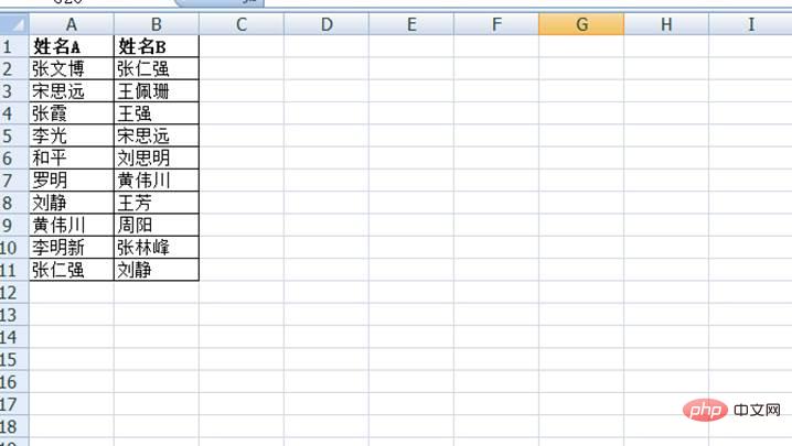
The operation method is to enter the formula =IF(COUNTIF(A:A,B2)=0,"",B2) in cell C2, and then pull down to complete the two columns of excel Data comparison. Please see the demo below!

The COUNTIF function is a function that counts cells in a specified range that meet specified conditions.

Test you:

If the numerical value compared above exceeds 15 digits, for example, the comparison is ID number, can the above formula still be used? If the above formula cannot be used, what about changing it to the following formula?

=IF(COUNTIF(A: A,B2&"*")=0," ",B2)

or

=IF(SUMPRODUCT(1*(A:A=B2)),B2,"")

If you don’t know the answer, please watch the tutorial " The card number is bizarre and reduced. My cousin was unjustly punished. ——Excel, it turns out you have duplicates of true and false! 》.

3) IF VLOOKUP function finds duplicate values

As shown in the table below, there are two sets of employee numbers. I don’t know which ones are common to both groups A and B. We can also use the if VLOOKUP function formula to complete the comparison.

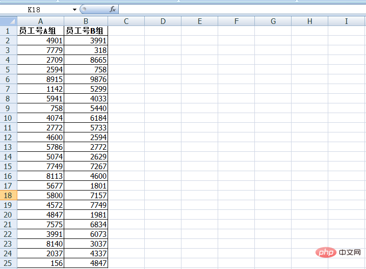
Enter the formula in cell C2: =IF(ISNA(VLOOKUP(A2,$B$2:$B$25,1,))," " ,A2), and then pull down to copy the formula, you can find the duplicate values ​​in the two columns of data in Excel.

Formula analysis:

The ISNA function is used to determine whether the value is an error value #N/A (that is, the value does not exist ), if yes, returns TRUE; otherwise returns FALSE.

In the formula, you need to add the $ sign before the data in the search area to fix the search area. Otherwise, the search area will also change when the drop-down is filled, which will affect the search and comparison results.

App Extension: Find Differences with Vlookup

This formula can be slightly adjusted to find different values, or missing values ​​or wrong values ​​(non-strict comparison, not paying attention to position or order). For example, the above group B is standard data. To find the values ​​in group A that are different from group B, the formula can be written as:

=IF(ISNA(VLOOKUP(A2,$B$2:$ B$25,1,)), A2, " ")

Part 2: Cross-table data comparison

1. Strictly compare whether the data of the two tables are the same

When two tables with exactly the same format are compared to find differences, the following method can be used.

1) Conditional formatting method to compare the differences between the two tables

Now take the following two tables as an example to compare which values ​​are different and highlight them.

First, select a table, create a new rule, and select "Use formulas to determine the cells to be formatted", then enter =A9A1, for the corresponding cells Make a judgment to determine whether they are equal. Please see the demo below!

Warm reminder:

If you want to clear conditional formatting, first select the cell range to clear the format, and then Execute "Start" - "Conditional Formatting" - "Clear Rules" - "Clear Rules for Selected Cells" (or clear the rules for the entire worksheet).

2) Compare the differences between the two tables using the special paste method (this method is only suitable for comparison of numbers)

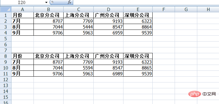
As shown in the figure below, the two tables have the same format and the same name ordering. It is required to quickly find the data differences between two tables.

Copy one of the numerical areas, then press the shortcut key Ctrl Alt V to paste selectively, set it to "subtraction" operation, click "OK", the non-0 part is The difference lies. Please see the demo below!

This method is only suitable for quickly locating differential data, just at a glance, because it will destroy the original data table.

3) IF function compares the differences between the two tables

As shown in the figure below, table a and table b are tables with exactly the same format. Now it is required to check the two tables Whether the values ​​​​are completely consistent, and the differences must be visually displayed.

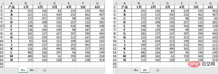
The operation method is to create a new blank worksheet and enter the formula =IF(Table a!A1 Table b!A1, "Table a:"& Table a!A1&" vs table b:"& table b!A1,""), then copy the fill formula within the range. Please see the demo below!

2. Find the difference between the data in the two tables according to conditions

1) Find the difference between the data in two tables using a single condition

For example, the following is a score table summarized by two people. The table format is the same, but the name ordering is different. Now you need to compare the two tables to verify whether the summary results are correct.

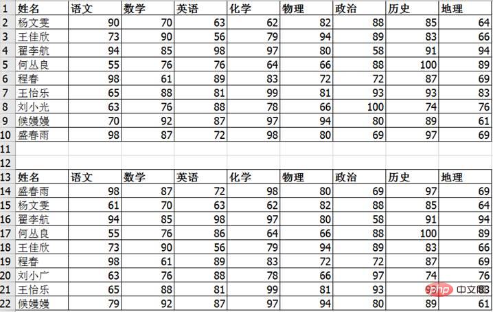
This type of data verification is a single condition verification. Because it is compiled by different people, in addition to checking the scores by name, it is also necessary to mark those whose names do not match. We do this using conditional formatting.

Two conditional formats need to be established.

The first format: Find the name difference

(1) Select the name column data of the second table, select "New Rule" in "Conditional Formatting", and in the pop-up In the dialog box, select "Use a formula to determine the cells to be formatted", and then enter the formula =COUNTIF($A$2:$A$10,A14)=0

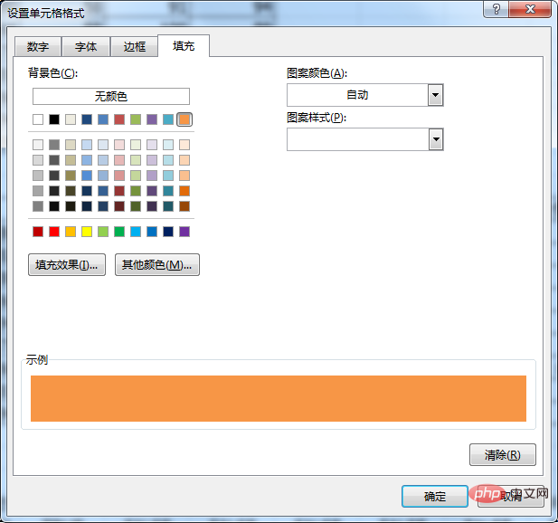
(2) Click the Format button and select A fill color.

After confirmation, we will complete the first format setting.

The second format: Find the difference in scores for the same name.

(1) Select all the score cells in the second table, create a new rule, and use the formula to determine the rule. The entered formula is = =VLOOKUP($A14,$A$1:$I$10,COLUMN(B1),0)-B14

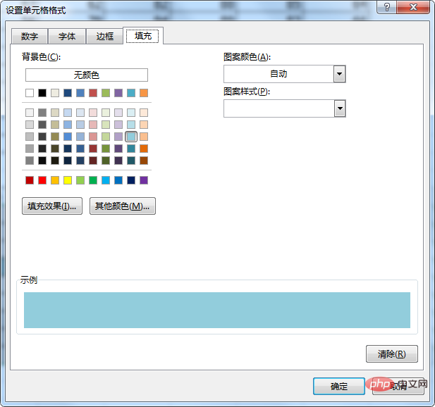
(2) Click the format button and select a fill color.

Complete the score check after confirmation. The overall verification results are as follows:

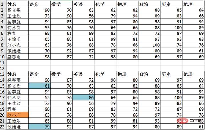
Orange indicates that the name "Liu Xiaoguang" does not match another table, and the name may be written incorrectly; blue-green indicates Yang Wenwen's Chinese score , He Congliang's English score, and Hou Manman's Chinese score do not match, and there may be errors.

2) Multiple conditions to find the difference in the data of the two tables

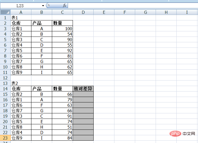
As shown in the figure below, it is required to check the quantity difference of the same product in the same warehouse in the two tables, and the results are shown In column D. In what way can this be accomplished? What a headache!

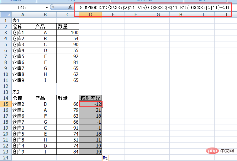
Enter the following formula in cell D15:

=SUMPRODUCT(($A$3:$A$11=A15)*($ B$3:$B$11=B15)*$C$3:$C$11)-C15

Then pull down to complete the comparison of the values. Please see please see! !

The above is today’s sharing, let’s practice together

Related learning recommendations: excel tutorial

The above is the detailed content of Practical Excel skills sharing: data comparison in several different situations. For more information, please follow other related articles on the PHP Chinese website!