
 Technology peripherals
AI
Comparative summary of ten nonlinear dimensionality reduction techniques in machine learning
Technology peripherals
AI
Comparative summary of ten nonlinear dimensionality reduction techniques in machine learning
Comparative summary of ten nonlinear dimensionality reduction techniques in machine learning

Dimensionality reduction refers to retaining the main information of the data as much as possible while reducing the number of features in the data set. Dimensionality reduction algorithms are unsupervised learning, and the algorithm is trained through unlabeled data.

Although there are many types of dimensionality reduction methods, they can all be classified into two major categories: linear and nonlinear.
Linear methods linearly project data from a high-dimensional space to a low-dimensional space (hence the name linear projection). Examples include PCA and LDA.
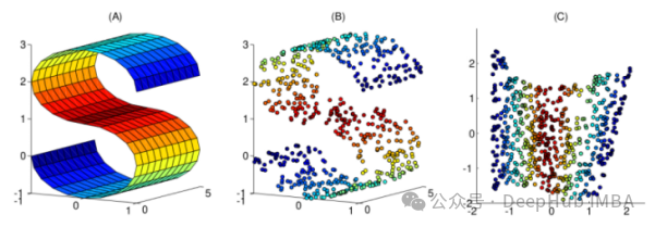
Nonlinear methods are a way to perform nonlinear dimensionality reduction, often used to discover the nonlinear structure of original data. Nonlinear dimensionality reduction methods are particularly important when the original data are not easily separated linearly. In some cases, nonlinear dimensionality reduction is also known as manifold learning. This method can handle high-dimensional data more efficiently and help reveal the underlying structure of the data. Through nonlinear dimensionality reduction, we can better understand the relationship between data, discover hidden patterns and rules in the data, and provide strong support for further data analysis and applications.
This article has compiled 10 commonly used nonlinear dimensionality reduction techniques, which can help you choose in your daily work
1. Kernel PCA
You may be familiar with normal PCA, which is a linear dimensionality reduction technique. Kernel PCA can be viewed as a nonlinear version of normal principal component analysis.
Both principal component analysis and kernel principal component analysis can be used for dimensionality reduction, but kernel PCA is more effective in processing linearly inseparable data. The main advantage of kernel PCA is to transform nonlinearly separable data into linearly separable data while reducing the data dimension. Kernel PCA can capture the nonlinear structure in the data by introducing kernel techniques, thereby improving the classification performance of the data. Therefore, kernel PCA has stronger expressiveness and generalization ability when dealing with complex data sets.
We first create a very classic data:
import matplotlib.pyplot as plt plt.figure(figsize=[7, 5]) from sklearn.datasets import make_moons X, y = make_moons(n_samples=100, noise=None, random_state=0) plt.scatter(X[:, 0], X[:, 1], c=y, s=50, cmap='plasma') plt.title('Linearly inseparable data')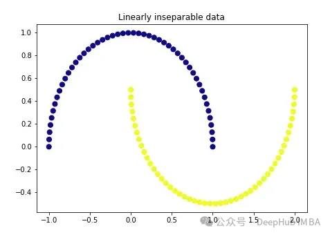
These two colors represent two linearly inseparable categories. It is impossible to draw a straight line here to separate these two categories.
We start with regular PCA.
import numpy as np from sklearn.decomposition import PCA pca = PCA(n_components=1) X_pca = pca.fit_transform(X) plt.figure(figsize=[7, 5]) plt.scatter(X_pca[:, 0], np.zeros((100,1)), c=y, s=50, cmap='plasma') plt.title('First component after linear PCA') plt.xlabel('PC1')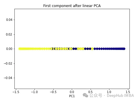
As you can see, the two classes are still linearly inseparable. Now let’s try kernel PCA.
import numpy as np from sklearn.decomposition import KernelPCA kpca = KernelPCA(n_components=1, kernel='rbf', gamma=15) X_kpca = kpca.fit_transform(X) plt.figure(figsize=[7, 5]) plt.scatter(X_kpca[:, 0], np.zeros((100,1)), c=y, s=50, cmap='plasma') plt.axvline(x=0.0, linestyle='dashed', color='black', linewidth=1.2) plt.title('First component after kernel PCA') plt.xlabel('PC1')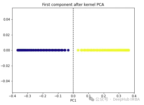
The two classes become linearly separable, and the kernel PCA algorithm uses different kernels to transform data from one form to the other. a form. Kernel PCA is a two-step process. First, the kernel function temporarily projects the original data into a high-dimensional space, where the classes are linearly separable. The algorithm then projects this data back to the lower dimensions specified in the n_components hyperparameter (the number of dimensions we want to preserve).
There are four kernel options in sklearn: linear’, ‘poly’, ‘rbf’ and ‘sigmoid’. If we specify the kernel as "linear", normal PCA will be performed. Any other kernel will perform nonlinear PCA. The rbf (radial basis function) kernel is the most commonly used.
2. Multidimensional scaling (MDS)
Multidimensional scaling is another nonlinear dimensionality reduction technique that maintains the distance between high-dimensional and low-dimensional data points. Perform dimensionality reduction. For example, points that are closer in the original dimension also appear closer in the lower dimensional form.
To use Scikit-learn we can use the MDS() class.
from sklearn.manifold import MDS mds = MDS(n_components, metric) mds_transformed = mds.fit_transform(X)
metric hyperparameters distinguish two types of MDS algorithms: metric and non-metric. If metric=True, execute metric MDS. Otherwise, perform non-metric MDS.
We apply two types of MDS algorithms to the following nonlinear data.
import numpy as np from sklearn.manifold import MDS mds = MDS(n_components=1, metric=True) # Metric MDS X_mds = mds.fit_transform(X) plt.figure(figsize=[7, 5]) plt.scatter(X_mds[:, 0], np.zeros((100,1)), c=y, s=50, cmap='plasma') plt.title('Metric MDS') plt.xlabel('Component 1')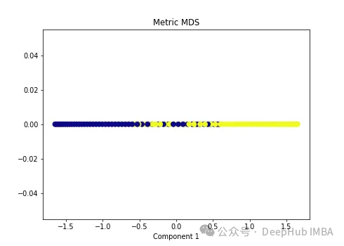
import numpy as np from sklearn.manifold import MDS mds = MDS(n_components=1, metric=False) # Non-metric MDS X_mds = mds.fit_transform(X) plt.figure(figsize=[7, 5]) plt.scatter(X_mds[:, 0], np.zeros((100,1)), c=y, s=50, cmap='plasma') plt.title('Non-metric MDS') plt.xlabel('Component 1')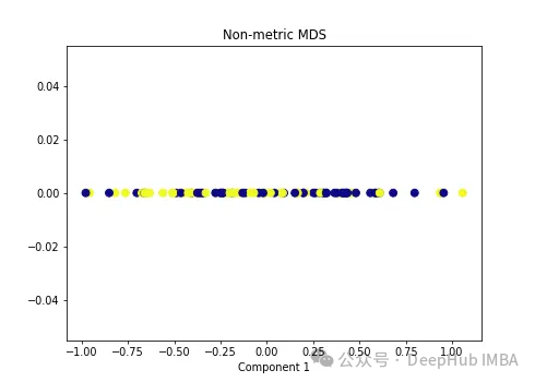
可以看到MDS后都不能使数据线性可分,所以可以说MDS不适合我们这个经典的数据集。
3、Isomap
Isomap(Isometric Mapping)在保持数据点之间的地理距离,即在原始高维空间中的测地线距离或者近似的测地线距离,在低维空间中也被保持。Isomap的基本思想是通过在高维空间中计算数据点之间的测地线距离(通过最短路径算法,比如Dijkstra算法),然后在低维空间中保持这些距离来进行降维。在这个过程中,Isomap利用了流形假设,即假设高维数据分布在一个低维流形上。因此,Isomap通常在处理非线性数据集时表现良好,尤其是当数据集包含曲线和流形结构时。
import matplotlib.pyplot as plt plt.figure(figsize=[7, 5]) from sklearn.datasets import make_moons X, y = make_moons(n_samples=100, noise=None, random_state=0) import numpy as np from sklearn.manifold import Isomap isomap = Isomap(n_neighbors=5, n_components=1) X_isomap = isomap.fit_transform(X) plt.figure(figsize=[7, 5]) plt.scatter(X_isomap[:, 0], np.zeros((100,1)), c=y, s=50, cmap='plasma') plt.title('First component after applying Isomap') plt.xlabel('Component 1')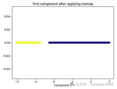
就像核PCA一样,这两个类在应用Isomap后是线性可分的!
4、Locally Linear Embedding(LLE)
与Isomap类似,LLE也是基于流形假设,即假设高维数据分布在一个低维流形上。LLE的主要思想是在局部邻域内保持数据点之间的线性关系,并在低维空间中重构这些关系。
from sklearn.manifold import LocallyLinearEmbedding lle = LocallyLinearEmbedding(n_neighbors=5,n_components=1) lle_transformed = lle.fit_transform(X) plt.figure(figsize=[7, 5]) plt.scatter(lle_transformed[:, 0], np.zeros((100,1)), c=y, s=50, cmap='plasma') plt.title('First component after applying LocallyLinearEmbedding') plt.xlabel('Component 1')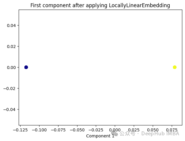
只有2个点,其实并不是这样,我们打印下这个数据
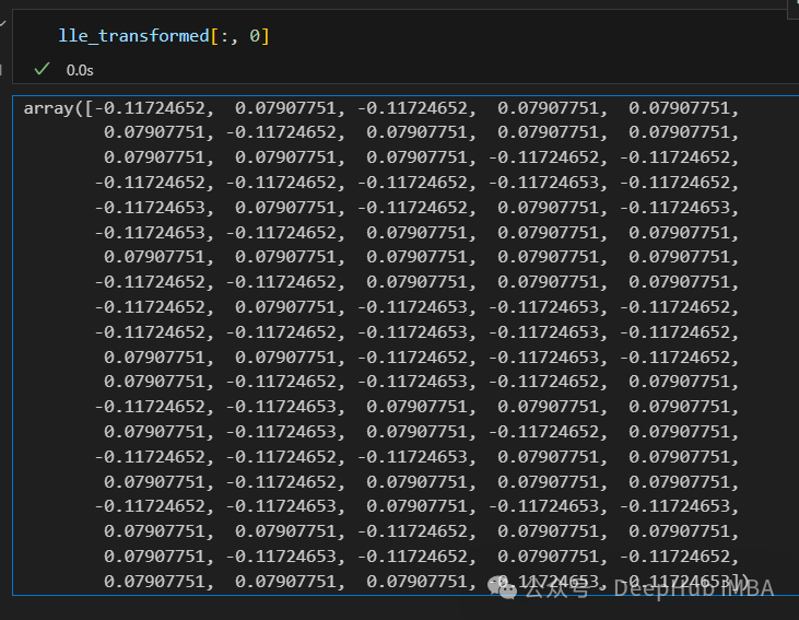
可以看到数据通过降维变成了同一个数字,所以LLE降维后是线性可分的,但是却丢失了数据的信息。
5、Spectral Embedding
Spectral Embedding是一种基于图论和谱理论的降维技术,通常用于将高维数据映射到低维空间。它的核心思想是利用数据的相似性结构,将数据点表示为图的节点,并通过图的谱分解来获取低维表示。
from sklearn.manifold import SpectralEmbedding sp_emb = SpectralEmbedding(n_components=1, affinity='nearest_neighbors') sp_emb_transformed = sp_emb.fit_transform(X) plt.figure(figsize=[7, 5]) plt.scatter(sp_emb_transformed[:, 0], np.zeros((100,1)), c=y, s=50, cmap='plasma') plt.title('First component after applying SpectralEmbedding') plt.xlabel('Component 1')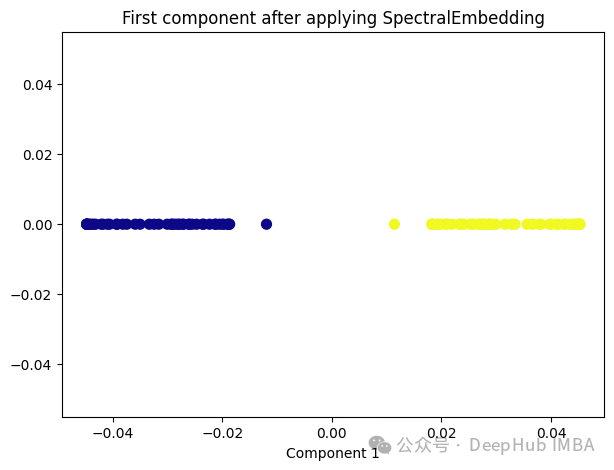
6、t-Distributed Stochastic Neighbor Embedding (t-SNE)
t-SNE的主要目标是保持数据点之间的局部相似性关系,并在低维空间中保持这些关系,同时试图保持全局结构。
from sklearn.manifold import TSNE tsne = TSNE(1, learning_rate='auto', init='pca') tsne_transformed = tsne.fit_transform(X) plt.figure(figsize=[7, 5]) plt.scatter(tsne_transformed[:, 0], np.zeros((100,1)), c=y, s=50, cmap='plasma') plt.title('First component after applying TSNE') plt.xlabel('Component 1')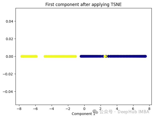
t-SNE好像也不太适合我们的数据。
7、Random Trees Embedding
Random Trees Embedding是一种基于树的降维技术,常用于将高维数据映射到低维空间。它利用了随机森林(Random Forest)的思想,通过构建多棵随机决策树来实现降维。
Random Trees Embedding的基本工作流程:
- 构建随机决策树集合:首先,构建多棵随机决策树。每棵树都是通过从原始数据中随机选择子集进行训练的,这样可以减少过拟合,提高泛化能力。
- 提取特征表示:对于每个数据点,通过将其在每棵树上的叶子节点的索引作为特征,构建一个特征向量。每个叶子节点都代表了数据点在树的某个分支上的位置。
- 降维:通过随机森林中所有树生成的特征向量,将数据点映射到低维空间中。通常使用降维技术,如主成分分析(PCA)或t-SNE等,来实现最终的降维过程。
Random Trees Embedding的优势在于它的计算效率高,特别是对于大规模数据集。由于使用了随机森林的思想,它能够很好地处理高维数据,并且不需要太多的调参过程。
RandomTreesEmbedding使用高维稀疏进行无监督转换,也就是说,我们最终得到的数据并不是一个连续的数值,而是稀疏的表示。所以这里就不进行代码展示了,有兴趣的看看sklearn的sklearn.ensemble.RandomTreesEmbedding
8、Dictionary Learning
Dictionary Learning是一种用于降维和特征提取的技术,它主要用于处理高维数据。它的目标是学习一个字典,该字典由一组原子(或基向量)组成,这些原子是数据的线性组合。通过学习这样的字典,可以将高维数据表示为一个更紧凑的低维空间中的稀疏线性组合。
Dictionary Learning的优点之一是它能够学习出具有可解释性的原子,这些原子可以提供关于数据结构和特征的重要见解。此外,Dictionary Learning还可以产生稀疏表示,从而提供更紧凑的数据表示,有助于降低存储成本和计算复杂度。
from sklearn.decomposition import DictionaryLearning dict_lr = DictionaryLearning(n_components=1) dict_lr_transformed = dict_lr.fit_transform(X) plt.figure(figsize=[7, 5]) plt.scatter(dict_lr_transformed[:, 0], np.zeros((100,1)), c=y, s=50, cmap='plasma') plt.title('First component after applying DictionaryLearning') plt.xlabel('Component 1')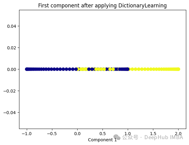
9、Independent Component Analysis (ICA)
Independent Component Analysis (ICA) 是一种用于盲源分离的统计方法,通常用于从混合信号中估计原始信号。在机器学习和信号处理领域,ICA经常用于解决以下问题:
- 盲源分离:给定一组混合信号,其中每个信号是一组原始信号的线性组合,ICA的目标是从混合信号中分离出原始信号,而不需要事先知道混合过程的具体细节。
- 特征提取:ICA可以被用来发现数据中的独立成分,提取数据的潜在结构和特征,通常在降维或预处理过程中使用。
ICA的基本假设是,混合信号中的各个成分是相互独立的,即它们的统计特性是独立的。这与主成分分析(PCA)不同,PCA假设成分之间是正交的,而不是独立的。因此ICA通常比PCA更适用于发现非高斯分布的独立成分。
from sklearn.decomposition import FastICA ica = FastICA(n_components=1, whiten='unit-variance') ica_transformed = dict_lr.fit_transform(X) plt.figure(figsize=[7, 5]) plt.scatter(ica_transformed[:, 0], np.zeros((100,1)), c=y, s=50, cmap='plasma') plt.title('First component after applying FastICA') plt.xlabel('Component 1')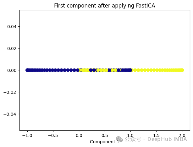
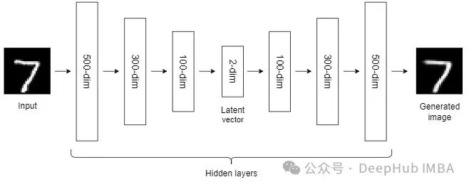
10、Autoencoders (AEs)
到目前为止,我们讨论的NLDR技术属于通用机器学习算法的范畴。而自编码器是一种基于神经网络的NLDR技术,可以很好地处理大型非线性数据。当数据集较小时,自动编码器的效果可能不是很好。
自编码器我们已经介绍过很多次了,所以这里就不详细说明了。
总结
非线性降维技术是一类用于将高维数据映射到低维空间的方法,它们通常适用于数据具有非线性结构的情况。
大多数NLDR方法基于最近邻方法,该方法要求数据中所有特征的尺度相同,所以如果特征的尺度不同,还需要进行缩放。
另外这些非线性降维技术在不同的数据集和任务中可能表现出不同的性能,因此在选择合适的方法时需要考虑数据的特征、降维的目标以及计算资源等因素。
The above is the detailed content of Comparative summary of ten nonlinear dimensionality reduction techniques in machine learning. For more information, please follow other related articles on the PHP Chinese website!

Hot AI Tools

Undresser.AI Undress
AI-powered app for creating realistic nude photos

AI Clothes Remover
Online AI tool for removing clothes from photos.

Undress AI Tool
Undress images for free

Clothoff.io
AI clothes remover

Video Face Swap
Swap faces in any video effortlessly with our completely free AI face swap tool!

Hot Article
Hot Tools

Notepad++7.3.1
Easy-to-use and free code editor

SublimeText3 Chinese version
Chinese version, very easy to use

Zend Studio 13.0.1
Powerful PHP integrated development environment

Dreamweaver CS6
Visual web development tools

SublimeText3 Mac version
God-level code editing software (SublimeText3)
Hot Topics
 1666
1666
 14
1425
52
1328
25
1273
29
1253
24
14
1425
52
1328
25
1273
29
1253
24

 15 recommended open source free image annotation tools
Mar 28, 2024 pm 01:21 PM
15 recommended open source free image annotation tools
Mar 28, 2024 pm 01:21 PM
Image annotation is the process of associating labels or descriptive information with images to give deeper meaning and explanation to the image content. This process is critical to machine learning, which helps train vision models to more accurately identify individual elements in images. By adding annotations to images, the computer can understand the semantics and context behind the images, thereby improving the ability to understand and analyze the image content. Image annotation has a wide range of applications, covering many fields, such as computer vision, natural language processing, and graph vision models. It has a wide range of applications, such as assisting vehicles in identifying obstacles on the road, and helping in the detection and diagnosis of diseases through medical image recognition. . This article mainly recommends some better open source and free image annotation tools. 1.Makesens
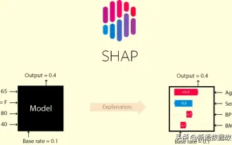 This article will take you to understand SHAP: model explanation for machine learning
Jun 01, 2024 am 10:58 AM
This article will take you to understand SHAP: model explanation for machine learning
Jun 01, 2024 am 10:58 AM
In the fields of machine learning and data science, model interpretability has always been a focus of researchers and practitioners. With the widespread application of complex models such as deep learning and ensemble methods, understanding the model's decision-making process has become particularly important. Explainable AI|XAI helps build trust and confidence in machine learning models by increasing the transparency of the model. Improving model transparency can be achieved through methods such as the widespread use of multiple complex models, as well as the decision-making processes used to explain the models. These methods include feature importance analysis, model prediction interval estimation, local interpretability algorithms, etc. Feature importance analysis can explain the decision-making process of a model by evaluating the degree of influence of the model on the input features. Model prediction interval estimate
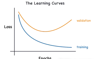 Identify overfitting and underfitting through learning curves
Apr 29, 2024 pm 06:50 PM
Identify overfitting and underfitting through learning curves
Apr 29, 2024 pm 06:50 PM
This article will introduce how to effectively identify overfitting and underfitting in machine learning models through learning curves. Underfitting and overfitting 1. Overfitting If a model is overtrained on the data so that it learns noise from it, then the model is said to be overfitting. An overfitted model learns every example so perfectly that it will misclassify an unseen/new example. For an overfitted model, we will get a perfect/near-perfect training set score and a terrible validation set/test score. Slightly modified: "Cause of overfitting: Use a complex model to solve a simple problem and extract noise from the data. Because a small data set as a training set may not represent the correct representation of all data." 2. Underfitting Heru
 The evolution of artificial intelligence in space exploration and human settlement engineering
Apr 29, 2024 pm 03:25 PM
The evolution of artificial intelligence in space exploration and human settlement engineering
Apr 29, 2024 pm 03:25 PM
In the 1950s, artificial intelligence (AI) was born. That's when researchers discovered that machines could perform human-like tasks, such as thinking. Later, in the 1960s, the U.S. Department of Defense funded artificial intelligence and established laboratories for further development. Researchers are finding applications for artificial intelligence in many areas, such as space exploration and survival in extreme environments. Space exploration is the study of the universe, which covers the entire universe beyond the earth. Space is classified as an extreme environment because its conditions are different from those on Earth. To survive in space, many factors must be considered and precautions must be taken. Scientists and researchers believe that exploring space and understanding the current state of everything can help understand how the universe works and prepare for potential environmental crises
 Transparent! An in-depth analysis of the principles of major machine learning models!
Apr 12, 2024 pm 05:55 PM
Transparent! An in-depth analysis of the principles of major machine learning models!
Apr 12, 2024 pm 05:55 PM
In layman’s terms, a machine learning model is a mathematical function that maps input data to a predicted output. More specifically, a machine learning model is a mathematical function that adjusts model parameters by learning from training data to minimize the error between the predicted output and the true label. There are many models in machine learning, such as logistic regression models, decision tree models, support vector machine models, etc. Each model has its applicable data types and problem types. At the same time, there are many commonalities between different models, or there is a hidden path for model evolution. Taking the connectionist perceptron as an example, by increasing the number of hidden layers of the perceptron, we can transform it into a deep neural network. If a kernel function is added to the perceptron, it can be converted into an SVM. this one
 Implementing Machine Learning Algorithms in C++: Common Challenges and Solutions
Jun 03, 2024 pm 01:25 PM
Implementing Machine Learning Algorithms in C++: Common Challenges and Solutions
Jun 03, 2024 pm 01:25 PM
Common challenges faced by machine learning algorithms in C++ include memory management, multi-threading, performance optimization, and maintainability. Solutions include using smart pointers, modern threading libraries, SIMD instructions and third-party libraries, as well as following coding style guidelines and using automation tools. Practical cases show how to use the Eigen library to implement linear regression algorithms, effectively manage memory and use high-performance matrix operations.
 Five schools of machine learning you don't know about
Jun 05, 2024 pm 08:51 PM
Five schools of machine learning you don't know about
Jun 05, 2024 pm 08:51 PM
Machine learning is an important branch of artificial intelligence that gives computers the ability to learn from data and improve their capabilities without being explicitly programmed. Machine learning has a wide range of applications in various fields, from image recognition and natural language processing to recommendation systems and fraud detection, and it is changing the way we live. There are many different methods and theories in the field of machine learning, among which the five most influential methods are called the "Five Schools of Machine Learning". The five major schools are the symbolic school, the connectionist school, the evolutionary school, the Bayesian school and the analogy school. 1. Symbolism, also known as symbolism, emphasizes the use of symbols for logical reasoning and expression of knowledge. This school of thought believes that learning is a process of reverse deduction, through existing
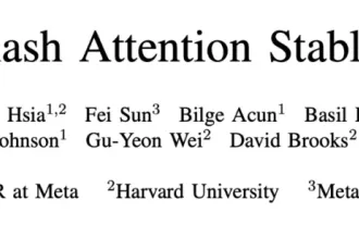 Is Flash Attention stable? Meta and Harvard found that their model weight deviations fluctuated by orders of magnitude
May 30, 2024 pm 01:24 PM
Is Flash Attention stable? Meta and Harvard found that their model weight deviations fluctuated by orders of magnitude
May 30, 2024 pm 01:24 PM
MetaFAIR teamed up with Harvard to provide a new research framework for optimizing the data bias generated when large-scale machine learning is performed. It is known that the training of large language models often takes months and uses hundreds or even thousands of GPUs. Taking the LLaMA270B model as an example, its training requires a total of 1,720,320 GPU hours. Training large models presents unique systemic challenges due to the scale and complexity of these workloads. Recently, many institutions have reported instability in the training process when training SOTA generative AI models. They usually appear in the form of loss spikes. For example, Google's PaLM model experienced up to 20 loss spikes during the training process. Numerical bias is the root cause of this training inaccuracy,
