
 Technology peripherals
AI
Ensemble methods for unsupervised learning: clustering of similarity matrices
Technology peripherals
AI
Ensemble methods for unsupervised learning: clustering of similarity matrices
Ensemble methods for unsupervised learning: clustering of similarity matrices

In machine learning, the term ensemble refers to combining multiple models in parallel. The idea is to use the wisdom of the crowd to form a better consensus on the final answer given.

In the field of supervised learning, this method has been widely studied and applied, especially in classification problems with very successful algorithms like RandomForest. A voting/weighting system is often employed to combine the output of each individual model into a more robust and consistent final output. In the world of unsupervised learning, this task becomes more difficult. First, because it encompasses the challenges of the field itself, we have no prior knowledge of the data to compare ourselves to any target. Second, because finding a suitable way to combine information from all models remains a problem, and there is no consensus on how to do this.
In this article, we discuss the best approach on this topic, namely clustering of similarity matrices.
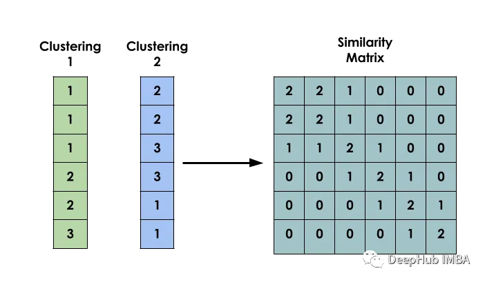 The main idea of this method is: given a data set X, create a matrix S such that Si represents the similarity between xi and xj. This matrix is constructed based on the clustering results of several different models.
Binary co-occurrence matrix
Creating a binary co-occurrence matrix between inputs is the first step in building a model
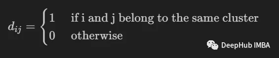 it Used to indicate whether two inputs i and j belong to the same cluster.
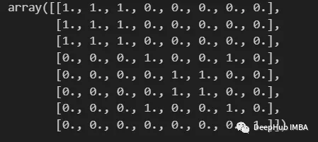
import numpy as np from scipy import sparse def build_binary_matrix( clabels ): data_len = len(clabels) matrix=np.zeros((data_len,data_len))for i in range(data_len):matrix[i,:] = clabels == clabels[i]return matrix labels = np.array( [1,1,1,2,3,3,2,4] ) build_binary_matrix(labels)
 Use KMeans to construct a similarity matrix
We have constructed a function to binarize our clustering, and now we can enter the stage of constructing the similarity matrix .
We introduce here a common method, which only involves calculating the average value between M co-occurrence matrices generated by M different models. We define it as:
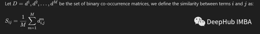 When the entries fall in the same cluster, their similarity value will be close to 1, while when the entries fall in different groups, Their similarity value will be close to 0
We will build a similarity matrix based on the labels created by the K-Means model. Conducted using the MNIST dataset. For simplicity and efficiency, we will only use 10,000 PCA-reduced images.
from sklearn.datasets import fetch_openml from sklearn.decomposition import PCA from sklearn.cluster import MiniBatchKMeans, KMeans from sklearn.model_selection import train_test_split mnist = fetch_openml('mnist_784') X = mnist.data y = mnist.target X, _, y, _ = train_test_split(X,y, train_size=10000, stratify=y, random_state=42 ) pca = PCA(n_components=0.99) X_pca = pca.fit_transform(X)To allow for diversity between models, each model is instantiated with a random number of clusters.
NUM_MODELS = 500 MIN_N_CLUSTERS = 2 MAX_N_CLUSTERS = 300 np.random.seed(214) model_sizes = np.random.randint(MIN_N_CLUSTERS, MAX_N_CLUSTERS+1, size=NUM_MODELS) clt_models = [KMeans(n_clusters=i, n_init=4, random_state=214) for i in model_sizes] for i, model in enumerate(clt_models):print( f"Fitting - {i+1}/{NUM_MODELS}" )model.fit(X_pca)The following function is to create a similarity matrix
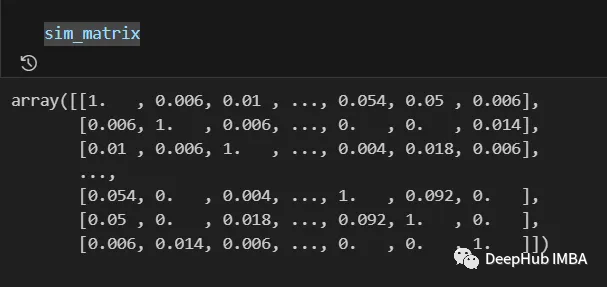
def build_similarity_matrix( models_labels ):n_runs, n_data = models_labels.shape[0], models_labels.shape[1] sim_matrix = np.zeros( (n_data, n_data) ) for i in range(n_runs):sim_matrix += build_binary_matrix( models_labels[i,:] ) sim_matrix = sim_matrix/n_runs return sim_matrix
Call this function:
models_labels = np.array([ model.labels_ for model in clt_models ]) sim_matrix = build_similarity_matrix(models_labels)
The final result is as follows:
 The information from the similarity matrix can still be post-processed before the last step, such as applying logarithmic, polynomial, etc. transformations.
In our case, we will keep the original intention unchanged and rewrite
Pos_sim_matrix = sim_matrix
Clustering the similarity matrix
The similarity matrix is a A way to represent the knowledge built by the collaboration of all clustering models.
We can use it to visually see which entries are more likely to belong to the same cluster and which ones do not. However, this information still needs to be converted into actual clusters. This is done by using a clustering algorithm that can receive a similarity matrix as a parameter. Here we use SpectralClustering.
from sklearn.cluster import SpectralClustering spec_clt = SpectralClustering(n_clusters=10, affinity='precomputed',n_init=5, random_state=214) final_labels = spec_clt.fit_predict(pos_sim_matrix)
Comparison with the standard KMeans model
Let’s compare it with KMeans to confirm whether our method is effective.
We will use NMI, ARI, cluster purity and class purity indicators to evaluate the standard KMeans model and compare with our ensemble model. Additionally, we will plot a contingency matrix to visualize which categories belong in each cluster
from seaborn import heatmap import matplotlib.pyplot as plt def data_contingency_matrix(true_labels, pred_labels): fig, (ax) = plt.subplots(1, 1, figsize=(8,8)) n_clusters = len(np.unique(pred_labels))n_classes = len(np.unique(true_labels))label_names = np.unique(true_labels)label_names.sort() contingency_matrix = np.zeros( (n_classes, n_clusters) ) for i, true_label in enumerate(label_names):for j in range(n_clusters):contingency_matrix[i, j] = np.sum(np.logical_and(pred_labels==j, true_labels==true_label)) heatmap(contingency_matrix.astype(int), ax=ax,annot=True, annot_kws={"fontsize":14}, fmt='d') ax.set_xlabel("Clusters", fontsize=18)ax.set_xticks( [i+0.5 for i in range(n_clusters)] )ax.set_xticklabels([i for i in range(n_clusters)], fontsize=14) ax.set_ylabel("Original classes", fontsize=18)ax.set_yticks( [i+0.5 for i in range(n_classes)] )ax.set_yticklabels(label_names, fontsize=14, va="center") ax.set_title("Contingency Matrix\n", ha='center', fontsize=20)from sklearn.metrics import normalized_mutual_info_score, adjusted_rand_score def purity( true_labels, pred_labels ): n_clusters = len(np.unique(pred_labels))n_classes = len(np.unique(true_labels))label_names = np.unique(true_labels) purity_vector = np.zeros( (n_classes) )contingency_matrix = np.zeros( (n_classes, n_clusters) ) for i, true_label in enumerate(label_names):for j in range(n_clusters):contingency_matrix[i, j] = np.sum(np.logical_and(pred_labels==j, true_labels==true_label)) purity_vector = np.max(contingency_matrix, axis=1)/np.sum(contingency_matrix, axis=1) print( f"Mean Class Purity - {np.mean(purity_vector):.2f}" ) for i, true_label in enumerate(label_names):print( f" {true_label} - {purity_vector[i]:.2f}" ) cluster_purity_vector = np.zeros( (n_clusters) )cluster_purity_vector = np.max(contingency_matrix, axis=0)/np.sum(contingency_matrix, axis=0) print( f"Mean Cluster Purity - {np.mean(cluster_purity_vector):.2f}" ) for i in range(n_clusters):print( f" {i} - {cluster_purity_vector[i]:.2f}" ) kmeans_model = KMeans(10, n_init=50, random_state=214) km_labels = kmeans_model.fit_predict(X_pca) data_contingency_matrix(y, km_labels) print( "Single KMeans NMI - ", normalized_mutual_info_score(y, km_labels) ) print( "Single KMeans ARI - ", adjusted_rand_score(y, km_labels) ) purity(y, km_labels)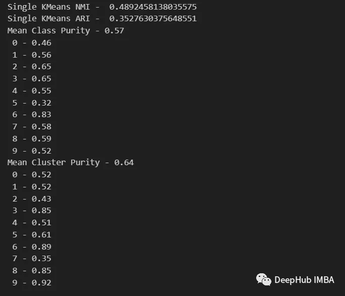
data_contingency_matrix(y, final_labels) print( "Ensamble NMI - ", normalized_mutual_info_score(y, final_labels) ) print( "Ensamble ARI - ", adjusted_rand_score(y, final_labels) ) purity(y, final_labels)
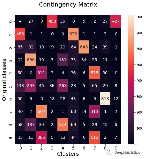
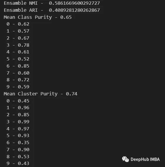
By observing the above values, it can be clearly seen that the Ensemble method can effectively improve the quality of clustering. At the same time, more consistent behavior can also be observed in the contingency matrix, with better distribution categories and less "noise"
The above is the detailed content of Ensemble methods for unsupervised learning: clustering of similarity matrices. For more information, please follow other related articles on the PHP Chinese website!

Hot AI Tools

Undresser.AI Undress
AI-powered app for creating realistic nude photos

AI Clothes Remover
Online AI tool for removing clothes from photos.

Undress AI Tool
Undress images for free

Clothoff.io
AI clothes remover

Video Face Swap
Swap faces in any video effortlessly with our completely free AI face swap tool!

Hot Article
Hot Tools

Notepad++7.3.1
Easy-to-use and free code editor

SublimeText3 Chinese version
Chinese version, very easy to use

Zend Studio 13.0.1
Powerful PHP integrated development environment

Dreamweaver CS6
Visual web development tools

SublimeText3 Mac version
God-level code editing software (SublimeText3)
Hot Topics
 1653
1653
 14
1413
52
1304
25
1251
29
1224
24
14
1413
52
1304
25
1251
29
1224
24

 15 recommended open source free image annotation tools
Mar 28, 2024 pm 01:21 PM
15 recommended open source free image annotation tools
Mar 28, 2024 pm 01:21 PM
Image annotation is the process of associating labels or descriptive information with images to give deeper meaning and explanation to the image content. This process is critical to machine learning, which helps train vision models to more accurately identify individual elements in images. By adding annotations to images, the computer can understand the semantics and context behind the images, thereby improving the ability to understand and analyze the image content. Image annotation has a wide range of applications, covering many fields, such as computer vision, natural language processing, and graph vision models. It has a wide range of applications, such as assisting vehicles in identifying obstacles on the road, and helping in the detection and diagnosis of diseases through medical image recognition. . This article mainly recommends some better open source and free image annotation tools. 1.Makesens
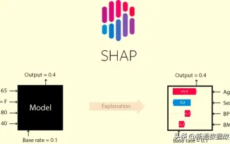 This article will take you to understand SHAP: model explanation for machine learning
Jun 01, 2024 am 10:58 AM
This article will take you to understand SHAP: model explanation for machine learning
Jun 01, 2024 am 10:58 AM
In the fields of machine learning and data science, model interpretability has always been a focus of researchers and practitioners. With the widespread application of complex models such as deep learning and ensemble methods, understanding the model's decision-making process has become particularly important. Explainable AI|XAI helps build trust and confidence in machine learning models by increasing the transparency of the model. Improving model transparency can be achieved through methods such as the widespread use of multiple complex models, as well as the decision-making processes used to explain the models. These methods include feature importance analysis, model prediction interval estimation, local interpretability algorithms, etc. Feature importance analysis can explain the decision-making process of a model by evaluating the degree of influence of the model on the input features. Model prediction interval estimate
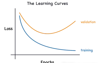 Identify overfitting and underfitting through learning curves
Apr 29, 2024 pm 06:50 PM
Identify overfitting and underfitting through learning curves
Apr 29, 2024 pm 06:50 PM
This article will introduce how to effectively identify overfitting and underfitting in machine learning models through learning curves. Underfitting and overfitting 1. Overfitting If a model is overtrained on the data so that it learns noise from it, then the model is said to be overfitting. An overfitted model learns every example so perfectly that it will misclassify an unseen/new example. For an overfitted model, we will get a perfect/near-perfect training set score and a terrible validation set/test score. Slightly modified: "Cause of overfitting: Use a complex model to solve a simple problem and extract noise from the data. Because a small data set as a training set may not represent the correct representation of all data." 2. Underfitting Heru
 The evolution of artificial intelligence in space exploration and human settlement engineering
Apr 29, 2024 pm 03:25 PM
The evolution of artificial intelligence in space exploration and human settlement engineering
Apr 29, 2024 pm 03:25 PM
In the 1950s, artificial intelligence (AI) was born. That's when researchers discovered that machines could perform human-like tasks, such as thinking. Later, in the 1960s, the U.S. Department of Defense funded artificial intelligence and established laboratories for further development. Researchers are finding applications for artificial intelligence in many areas, such as space exploration and survival in extreme environments. Space exploration is the study of the universe, which covers the entire universe beyond the earth. Space is classified as an extreme environment because its conditions are different from those on Earth. To survive in space, many factors must be considered and precautions must be taken. Scientists and researchers believe that exploring space and understanding the current state of everything can help understand how the universe works and prepare for potential environmental crises
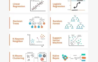 Transparent! An in-depth analysis of the principles of major machine learning models!
Apr 12, 2024 pm 05:55 PM
Transparent! An in-depth analysis of the principles of major machine learning models!
Apr 12, 2024 pm 05:55 PM
In layman’s terms, a machine learning model is a mathematical function that maps input data to a predicted output. More specifically, a machine learning model is a mathematical function that adjusts model parameters by learning from training data to minimize the error between the predicted output and the true label. There are many models in machine learning, such as logistic regression models, decision tree models, support vector machine models, etc. Each model has its applicable data types and problem types. At the same time, there are many commonalities between different models, or there is a hidden path for model evolution. Taking the connectionist perceptron as an example, by increasing the number of hidden layers of the perceptron, we can transform it into a deep neural network. If a kernel function is added to the perceptron, it can be converted into an SVM. this one
 Implementing Machine Learning Algorithms in C++: Common Challenges and Solutions
Jun 03, 2024 pm 01:25 PM
Implementing Machine Learning Algorithms in C++: Common Challenges and Solutions
Jun 03, 2024 pm 01:25 PM
Common challenges faced by machine learning algorithms in C++ include memory management, multi-threading, performance optimization, and maintainability. Solutions include using smart pointers, modern threading libraries, SIMD instructions and third-party libraries, as well as following coding style guidelines and using automation tools. Practical cases show how to use the Eigen library to implement linear regression algorithms, effectively manage memory and use high-performance matrix operations.
 Five schools of machine learning you don't know about
Jun 05, 2024 pm 08:51 PM
Five schools of machine learning you don't know about
Jun 05, 2024 pm 08:51 PM
Machine learning is an important branch of artificial intelligence that gives computers the ability to learn from data and improve their capabilities without being explicitly programmed. Machine learning has a wide range of applications in various fields, from image recognition and natural language processing to recommendation systems and fraud detection, and it is changing the way we live. There are many different methods and theories in the field of machine learning, among which the five most influential methods are called the "Five Schools of Machine Learning". The five major schools are the symbolic school, the connectionist school, the evolutionary school, the Bayesian school and the analogy school. 1. Symbolism, also known as symbolism, emphasizes the use of symbols for logical reasoning and expression of knowledge. This school of thought believes that learning is a process of reverse deduction, through existing
 Is Flash Attention stable? Meta and Harvard found that their model weight deviations fluctuated by orders of magnitude
May 30, 2024 pm 01:24 PM
Is Flash Attention stable? Meta and Harvard found that their model weight deviations fluctuated by orders of magnitude
May 30, 2024 pm 01:24 PM
MetaFAIR teamed up with Harvard to provide a new research framework for optimizing the data bias generated when large-scale machine learning is performed. It is known that the training of large language models often takes months and uses hundreds or even thousands of GPUs. Taking the LLaMA270B model as an example, its training requires a total of 1,720,320 GPU hours. Training large models presents unique systemic challenges due to the scale and complexity of these workloads. Recently, many institutions have reported instability in the training process when training SOTA generative AI models. They usually appear in the form of loss spikes. For example, Google's PaLM model experienced up to 20 loss spikes during the training process. Numerical bias is the root cause of this training inaccuracy,
