Sharing practical Excel skills: Understand the classic formula for extracting mobile phone numbers!

How to quickly extract mobile phone numbers in excel has become a common topic. After the advent of CTRL E, the problems of extracting data have become much simpler. I have to admit that it is indeed a very excellent function. But it is not a panacea, and there are still some data extraction problems that require formulas to solve. Next, the veteran rookie will explain to you the common formulas for extracting mobile phone numbers in Excel, and lead you to analyze the formulas in depth. Come and take a look~

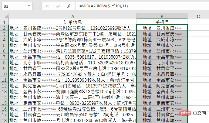
After Double 11 , everyone is busy tossing about their orders. While receiving a large number of orders, the workload of the girls in the customer service department is also much greater, especially the work of extracting customer mobile phone numbers from some more troublesome data, which is even more frustrating. People have a headache, for example, the following table:

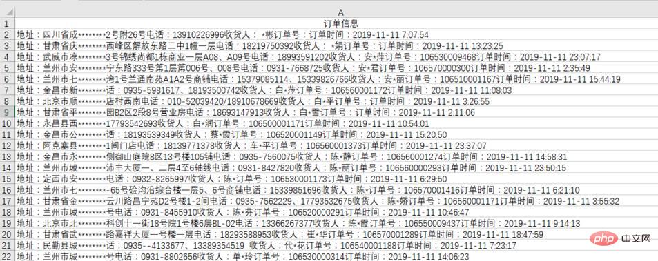
(The order information content is simulated data)

When encountering such data, I complain about the unreasonableness of the system. At the same time, I have to find a way to extract the mobile phone number, which is thousands of rows of data...

I heard that there seems to be a shortcut key called Ctrl E that can extract the phone number, try it quickly:

It seems that when encountering such complex data, the Ctrl E method known as smart filling also fails. What should I do?

VBA......

Absolutely no, is there any way to save it?

In fact, there is a formula that can solve this problem. The formula is:

=LOOKUP(9E 307,--MID(LEFT(A2,FIND("Consignee", A2)),ROW($1:$99),11))

The result is as shown in the figure:

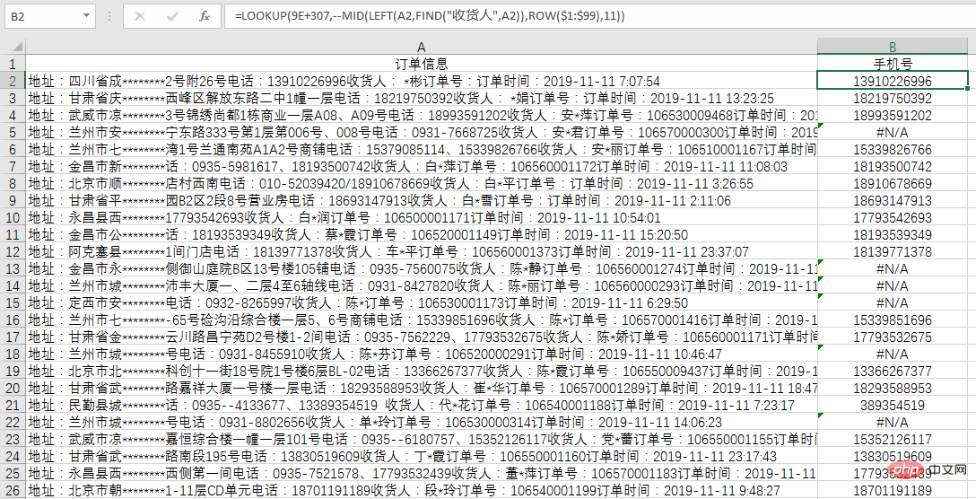
The formula does not look very long , but five functions are used for combination. Let’s break down the principle of this formula.

To solve the problem, we must first find the pattern. One feature of the mobile phone number is that it is 11 digits in length, and all of them are numbers. Therefore, you can use the routine of extracting numbers to solve the problem.

The difference from the usual problem of extracting numbers is that in these order information, the position of the mobile phone number is not fixed, and there will be other digital interference. The only thing that can be used is the 11-digit number. .

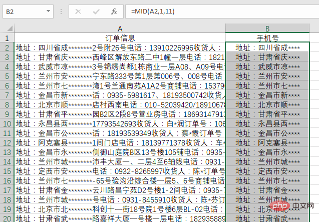
This requires the use of the MID function. The format is: MID(A2,1,11), which means starting from the first word in cell A2, intercept 11 words. The formula result is:

This is easy to understand. Since the starting position of the mobile phone number is not sure, a common routine is to use ROW as the second parameter of the MID function to achieve multiple extractions. To facilitate the understanding of the effect, ROW (1:10) is first used for explanation.

Let’s take a look at the effect of the formula =MID(A2,ROW(1:10),11):

Look at it this way There is no difference, but after checking it through the F9 function, you will find that 10 intercepted contents are obtained:

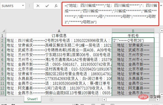
This formula is equivalent to MID(A2,1,11) , MID(A2,2,11)...MID(A2,10,11) effect.

In order to extract the mobile phone number, we must continue to enlarge the second parameter of the MID. It is customary to use ROW (1:99). Let’s take a look at the effect:

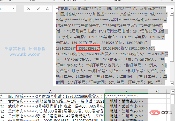
You can see that the mobile phone number is indeed in this large string of characters.

At this point, the mobile phone number has been successfully intercepted. The next step is how to get the required mobile phone number from this set of strings.

At this time, LOOKUP needs to come into play. The original formula should be written as: =LOOKUP(9E307,--MID(A2,ROW($1:$99),11)).

9E307 represents a very large number. Adding "--" before MID means converting the intercepted content into numbers. The principle of this formula has been explained many times in previous tutorials.

But the result obtained by the formula is surprising:

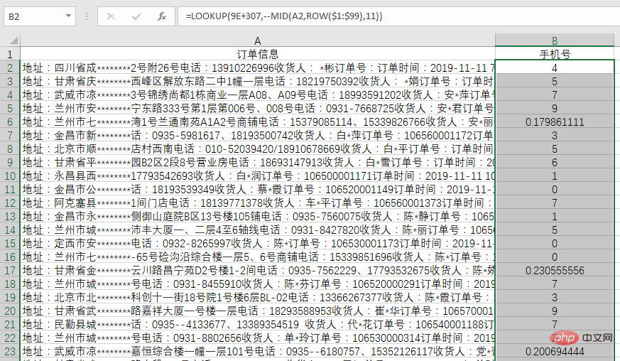
This is because the LOOKUP function obtains the number that appears in the last position. In the case of the data , in addition to the mobile phone number, the order time also appears, so in order to get the final result, the last step is needed to narrow the scope of LOOKUP processing.

Looking at the data source again, we can find a pattern. The mobile phone number is always before the "consignee", so we only need to extract the string in front of the consignee, and then use the formula just now. Can get results.

This is very easy to achieve. It can be completed using the LEFT FIND combination. The formula is: =LEFT(A2,FIND("Consignee",A2)). The result is as shown in the figure:

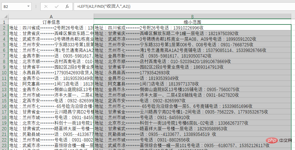
The LEFT FIND combination is easier to understand. If you have any questions, please leave a message. We will compile a tutorial on several similar common combinations.

Now substitute the narrowed range result into the previous formula, and you will have the final formula: =LOOKUP(9E 307,--MID(LEFT(A2,FIND("Consignee",A2)) ,ROW($1:$99),11))

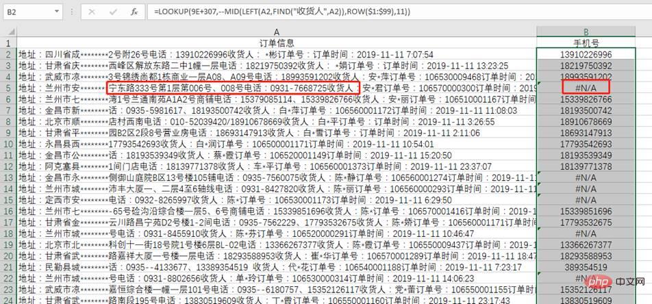
The result is an error value indicating that there is no mobile phone number in the order information.

Summary: The principle of this formula has been analyzed for everyone. From today's case, you can learn how to split a seemingly complex problem. The method is to find the rules and regularities bit by bit. The stronger you are, the more solutions you have.

In fact, there is another way to think about this problem, which is to use the formula:

=MAX(IFERROR(--MID(LEFT(A2,FIND("Collect",A2)) ,ROW($1:$99),11),0)) to complete.

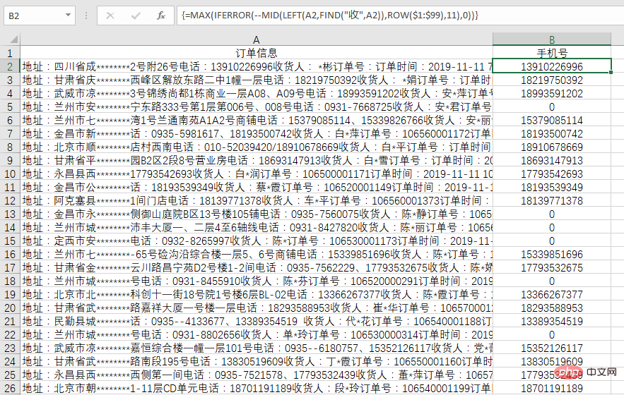
#Interested partners can try to analyze the principles of the formula by themselves. Of course, you can also leave a message to see what everyone needs and I will talk about this formula again.

Related learning recommendations: excel tutorial

The above is the detailed content of Sharing practical Excel skills: Understand the classic formula for extracting mobile phone numbers!. For more information, please follow other related articles on the PHP Chinese website!