
 Topics
excel
Practical Excel skills sharing: 10 most commonly used formulas among professionals
Topics
excel
Practical Excel skills sharing: 10 most commonly used formulas among professionals
Practical Excel skills sharing: 10 most commonly used formulas among professionals

This article has compiled 10 of the most commonly used excel formulas for professionals. I hope it can help you solve your problems. Come and take a look!

Formula 1: Conditional Counting
Conditional counting is very common in Excel applications. For example, the number of women in the statistical list of personnel is the condition. Typical representation of counting.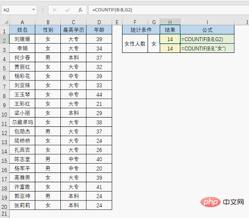
=COUNTIF (statistical area, condition). In this example, the first formula =COUNTIF(B:B,G2), B:B is the statistical area, G2 is the condition, and the formula result indicates that there are 14 "female" data in column B.
= COUNTIF(B:B,"女")That's it.
Formula 2: Quickly mark duplicate data
In daily work, we often encounter the problem of marking duplicate values, for example, in a document In the sales detail table, mark the duplicate salesperson names.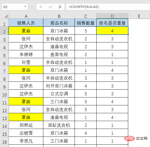
=COUNTIF(A:A,A2) to calculate the number of times each name appears. When the result is greater than 1, it means that the name is repeated. , and then use the IF function to get the final result.
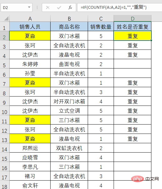
=IF(COUNTIF(A:A,A2)=1,"","Repeat"), the result is as shown in the figure.
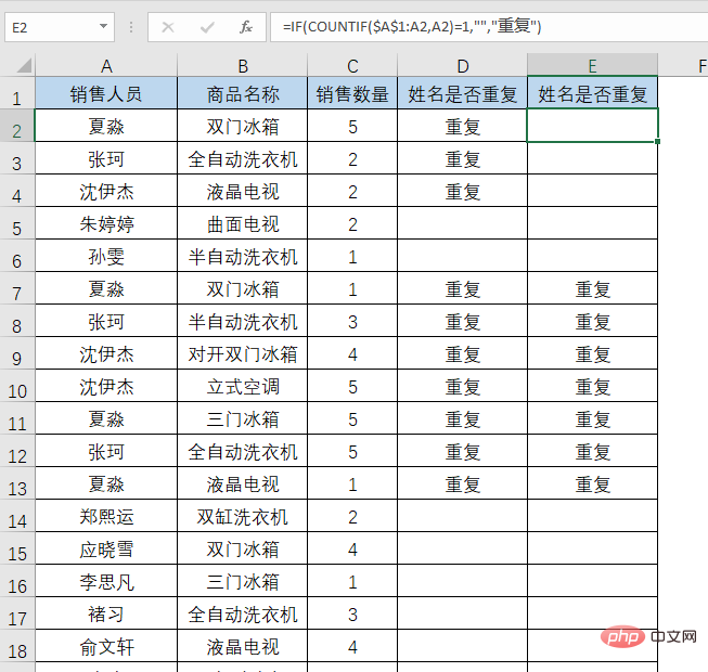
=IF(COUNTIF($A$1:A2,A2)=1,"","Repeat "), the result is as shown in the figure.
Formula 3: Multi-condition counting
If you want to count multiple conditions, you must Use the COUNTIFS function, for example, you need to count the number of men with a bachelor's degree in secondary school.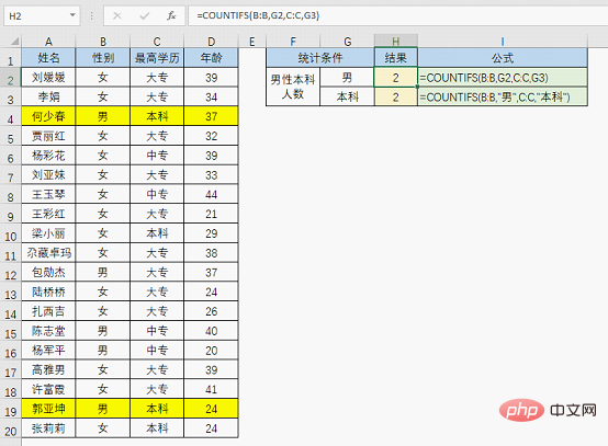
Formula 4: Conditional summation
In addition to conditional counting, conditional summation is also widely used, such as statistics in sales details Total TV sales.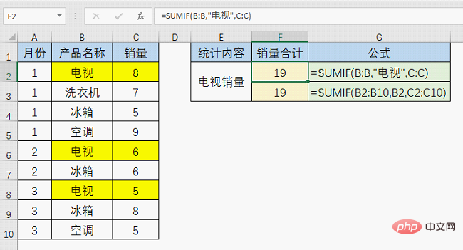
=SUMIF(B:B,B2,C:C).
Formula 5: Multi-condition summation
If there is a conditional summation, there will be a multi-condition summation, for example, based on salesperson and product When summing two conditions, the multi-condition summation function SUMIFS is used.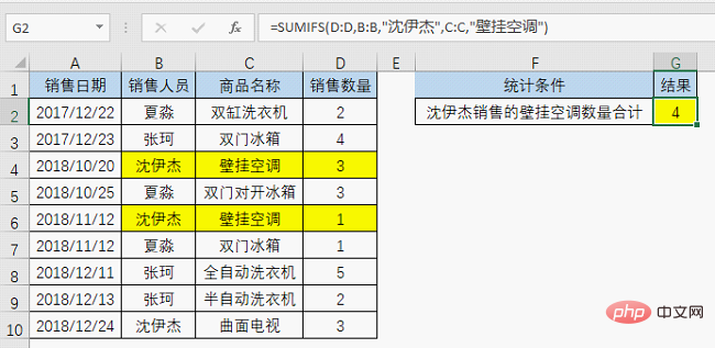
= SUMIFS(D:D,B:B,"Shen Yijie",C:C,"Wall-mounted air conditioner")
It should be reminded that the location of the summation area of SUMIFS is different from that of SUMIF. The summation area of SUMIFS is in the first parameter, while the summation area of SUMIF is in the third parameter. Don't get confused!
Formula 6: Calculate the date of birth based on the ID number
To get the date of birth from the ID number, this problem is very difficult for people who work Friends who are in administrative positions must be familiar with it, and the formula is relatively simple:
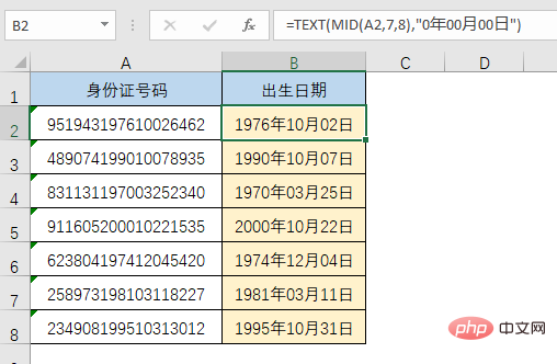
=TEXT(MID(A2,7,8),"0-00-00") to get the required results, as shown in the figure Shown:
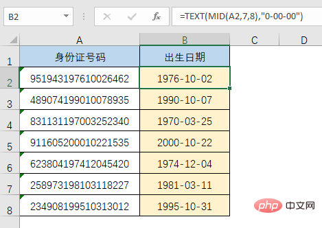
To understand the principle of this formula, you must first know some rules in ID numbers. The ID cards currently used are basically 18 digits. The eight digits starting with the seven digits represent the date of birth.
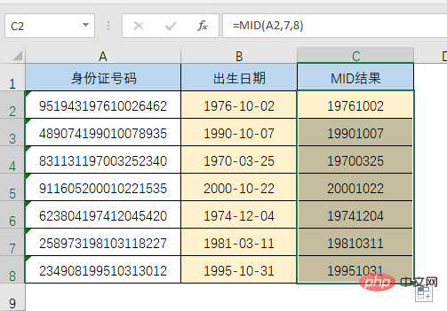
This formula involves two functions. First, let’s look at the MID function. The MID function has three parameters. The format is: =MID (where to extract, from which word to start, how many words to pick) .
MID(A2,7,8) means to intercept eight digits starting from the seventh number of cell A2. The effect is as shown in the figure:
After the birth date is extracted, it is not the effect we need. At this time, the function magician TEXT comes into play. The TEXT function has only two parameters, the format is =TEXT (the content to be processed, "in what format to display"), in this example The content to be processed is the MID function part. The display format is "0-00-00". Of course, it is no problem if you use the format of "0年00月00日". The formula is changed to =TEXT(MID(A2 ,7,8),"0年00月00日") will do:
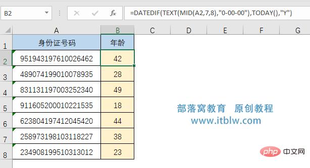
##Formula 7: Calculate age based on ID number
With the date of birth, of course you will think of calculating age. The formula is: =DATEDIF(B2,TODAY(),"Y")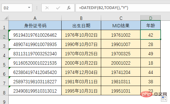
Formula 8: Different results are obtained according to the interval
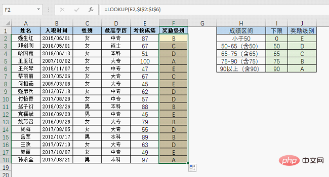
This type of problem is often seen in performance appraisals. For example, when a company conducts performance appraisals for employees, it needs to determine the reward level based on the appraisal results. The grading rules are: E for scores below 50, D for 50-65 (inclusive), and D for 65-75 (inclusive). ) is C, 75-90 (inclusive) is B, and above 90 is A. You can use the formula =LOOKUP(E2,{0;50;65;75;90},{"E";"D";"C";"B";"A"}) to get each The reward level of each employee, the result is as shown in the figure: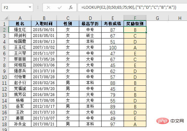
Formula 9: Single condition matching data
If you want to dominate the workplace, what can you do if you don’t know how to match? ? How can I do single condition matching without VLOOKUP? The basic structure of the VLOOKUP function is =VLOOKUP (what to look for, where to look for it, which column to look for, how to look for it). For example, to find the highest educational level by name, you can use the formula =VLOOKUP(G2,B:E,4 ,0) Get the desired result, as shown in the figure: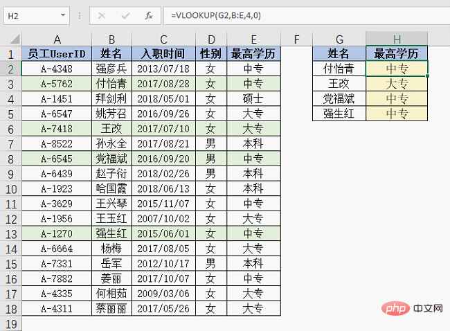
②The column number refers to the column in the search range rather than the column in the table. For example, if you want to find the highest educational level, you should find the 4th column in the search range, not the column number 5 in the table.
Formula 10: Multi-condition matching data
If you learn to match data with multiple conditions, you will be truly invincible!
Give an example of matching sales quantity by name and product name, as shown in the figure:

The formula is =LOOKUP( 1,0/(($A$2:$A$10=E2)*($B$2:$B$10=F2)),$C$2:$C$10)
Use the LOOKUP function The routine for multi-condition matching is: =LOOKUP(1,0/((search range 1=lookup value 1)*(search range 2=lookup value 2)*……*(search range n=lookup value n)), Result range), it should be noted that there is a multiplication relationship between multiple search conditions, and they need to be placed in the same set of brackets as the denominator of 0/.
Okay, the ten most commonly used formulas are shared here. If you use them well, you can really dominate the workplace!
Related learning recommendations: excel tutorial
The above is the detailed content of Practical Excel skills sharing: 10 most commonly used formulas among professionals. For more information, please follow other related articles on the PHP Chinese website!

Hot AI Tools

Undresser.AI Undress
AI-powered app for creating realistic nude photos

AI Clothes Remover
Online AI tool for removing clothes from photos.

Undress AI Tool
Undress images for free

Clothoff.io
AI clothes remover

Video Face Swap
Swap faces in any video effortlessly with our completely free AI face swap tool!

Hot Article
Hot Tools

Notepad++7.3.1
Easy-to-use and free code editor

SublimeText3 Chinese version
Chinese version, very easy to use

Zend Studio 13.0.1
Powerful PHP integrated development environment

Dreamweaver CS6
Visual web development tools

SublimeText3 Mac version
God-level code editing software (SublimeText3)
Hot Topics


 What should I do if the frame line disappears when printing in Excel?
Mar 21, 2024 am 09:50 AM
What should I do if the frame line disappears when printing in Excel?
Mar 21, 2024 am 09:50 AM
If when opening a file that needs to be printed, we will find that the table frame line has disappeared for some reason in the print preview. When encountering such a situation, we must deal with it in time. If this also appears in your print file If you have questions like this, then join the editor to learn the following course: What should I do if the frame line disappears when printing a table in Excel? 1. Open a file that needs to be printed, as shown in the figure below. 2. Select all required content areas, as shown in the figure below. 3. Right-click the mouse and select the "Format Cells" option, as shown in the figure below. 4. Click the “Border” option at the top of the window, as shown in the figure below. 5. Select the thin solid line pattern in the line style on the left, as shown in the figure below. 6. Select "Outer Border"
 How to filter more than 3 keywords at the same time in excel
Mar 21, 2024 pm 03:16 PM
How to filter more than 3 keywords at the same time in excel
Mar 21, 2024 pm 03:16 PM
Excel is often used to process data in daily office work, and it is often necessary to use the "filter" function. When we choose to perform "filtering" in Excel, we can only filter up to two conditions for the same column. So, do you know how to filter more than 3 keywords at the same time in Excel? Next, let me demonstrate it to you. The first method is to gradually add the conditions to the filter. If you want to filter out three qualifying details at the same time, you first need to filter out one of them step by step. At the beginning, you can first filter out employees with the surname "Wang" based on the conditions. Then click [OK], and then check [Add current selection to filter] in the filter results. The steps are as follows. Similarly, perform filtering separately again
 How to change excel table compatibility mode to normal mode
Mar 20, 2024 pm 08:01 PM
How to change excel table compatibility mode to normal mode
Mar 20, 2024 pm 08:01 PM
In our daily work and study, we copy Excel files from others, open them to add content or re-edit them, and then save them. Sometimes a compatibility check dialog box will appear, which is very troublesome. I don’t know Excel software. , can it be changed to normal mode? So below, the editor will bring you detailed steps to solve this problem, let us learn together. Finally, be sure to remember to save it. 1. Open a worksheet and display an additional compatibility mode in the name of the worksheet, as shown in the figure. 2. In this worksheet, after modifying the content and saving it, the dialog box of the compatibility checker always pops up. It is very troublesome to see this page, as shown in the figure. 3. Click the Office button, click Save As, and then
 How to set superscript in excel
Mar 20, 2024 pm 04:30 PM
How to set superscript in excel
Mar 20, 2024 pm 04:30 PM
When processing data, sometimes we encounter data that contains various symbols such as multiples, temperatures, etc. Do you know how to set superscripts in Excel? When we use Excel to process data, if we do not set superscripts, it will make it more troublesome to enter a lot of our data. Today, the editor will bring you the specific setting method of excel superscript. 1. First, let us open the Microsoft Office Excel document on the desktop and select the text that needs to be modified into superscript, as shown in the figure. 2. Then, right-click and select the "Format Cells" option in the menu that appears after clicking, as shown in the figure. 3. Next, in the “Format Cells” dialog box that pops up automatically
 How to use the iif function in excel
Mar 20, 2024 pm 06:10 PM
How to use the iif function in excel
Mar 20, 2024 pm 06:10 PM
Most users use Excel to process table data. In fact, Excel also has a VBA program. Apart from experts, not many users have used this function. The iif function is often used when writing in VBA. It is actually the same as if The functions of the functions are similar. Let me introduce to you the usage of the iif function. There are iif functions in SQL statements and VBA code in Excel. The iif function is similar to the IF function in the excel worksheet. It performs true and false value judgment and returns different results based on the logically calculated true and false values. IF function usage is (condition, yes, no). IF statement and IIF function in VBA. The former IF statement is a control statement that can execute different statements according to conditions. The latter
 How to type subscript in excel
Mar 20, 2024 am 11:31 AM
How to type subscript in excel
Mar 20, 2024 am 11:31 AM
eWe often use Excel to make some data tables and the like. Sometimes when entering parameter values, we need to superscript or subscript a certain number. For example, mathematical formulas are often used. So how do you type the subscript in Excel? ?Let’s take a look at the detailed steps: 1. Superscript method: 1. First, enter a3 (3 is superscript) in Excel. 2. Select the number "3", right-click and select "Format Cells". 3. Click "Superscript" and then "OK". 4. Look, the effect is like this. 2. Subscript method: 1. Similar to the superscript setting method, enter "ln310" (3 is the subscript) in the cell, select the number "3", right-click and select "Format Cells". 2. Check "Subscript" and click "OK"
 Where to set excel reading mode
Mar 21, 2024 am 08:40 AM
Where to set excel reading mode
Mar 21, 2024 am 08:40 AM
In the study of software, we are accustomed to using excel, not only because it is convenient, but also because it can meet a variety of formats needed in actual work, and excel is very flexible to use, and there is a mode that is convenient for reading. Today I brought For everyone: where to set the excel reading mode. 1. Turn on the computer, then open the Excel application and find the target data. 2. There are two ways to set the reading mode in Excel. The first one: In Excel, there are a large number of convenient processing methods distributed in the Excel layout. In the lower right corner of Excel, there is a shortcut to set the reading mode. Find the pattern of the cross mark and click it to enter the reading mode. There is a small three-dimensional mark on the right side of the cross mark.
 How to insert excel icons into PPT slides
Mar 26, 2024 pm 05:40 PM
How to insert excel icons into PPT slides
Mar 26, 2024 pm 05:40 PM
1. Open the PPT and turn the page to the page where you need to insert the excel icon. Click the Insert tab. 2. Click [Object]. 3. The following dialog box will pop up. 4. Click [Create from file] and click [Browse]. 5. Select the excel table to be inserted. 6. Click OK and the following page will pop up. 7. Check [Show as icon]. 8. Click OK.
