

Practical Excel skills sharing: Use Vlookup to compare multiple columns of data

How to compare multiple columns of data! When it comes to comparing multiple columns of data, it’s actually not difficult to say, nor easy to say. Before learning, I need to introduce you to a new friend, VLOOKUP, so let’s take a look together!

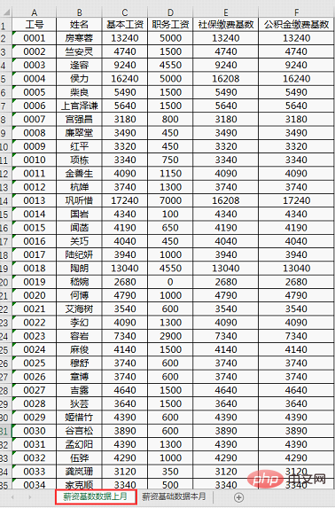
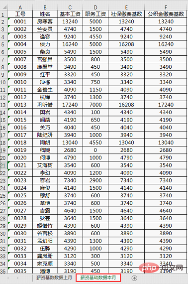
In the last study, we learned that we can use the merge calculation function to compare single column data. We compared names based on job numbers to find out the changes in personnel. Today we are going to compare four columns of data: basic salary, job salary, social security, and provident fund. It is a comparison of multiple columns of data.
##Last month’s data #We can also use merged calculations to compare multiple columns of data. Please think about and experiment with how to merge and compare data. What the editor here wants to share with you is another Super 6 method, which can quickly compare the differences between data! That's right, that's it - the VLOOKUP function! It is the most popular function in Excel~VLOOKUP is a search function. Its main function is to return the value at the intersection of the specified column in the search area and the row where the value is being found. Function structure:
VLOOKUP(查找啥,在哪查,返回第几列,0)
##What to look for
: That is the value to be found~Where is-
Search
: That is, the area to be searched ~ -
Which column to return
: That is, which column to return the data in the search area ~ -
Exact search/Approximate search
: Generally we search exactly, the default value is 0; if it is an approximate search, the default value is 1 After reading the above introduction, are you a little confused? Don’t worry, you will all understand with an example!
The following is the time to raise chestnuts.
There are two tables. The first table only has the work number but no name, while the second table is complete and contains both the work number and the name. We want to use the data in Table 2 to fill in the name column in Table 1. In other words, the job number is searched in Table 2, and then the name corresponding to the job number is returned to Table 1.

The formula should be like this:
=VLOOKUP(B4,E$4:F$9,2,0)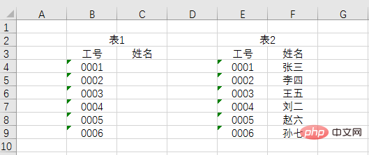
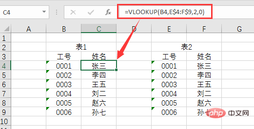
② Where to search: We need to search in the E4:F9 area of Table 2. At the same time, in order to keep the search area unchanged when the formula is filled down, we must add an absolute reference symbol to lock the number of rows, so the search area is E$4:F$9
③ Which column to return: We need to return the name column in Table 2, and the name column is the second column in the E:F area, so it is the number 2④ 0: Here we To achieve accurate search, the default value is 0After looking at the above examples, I believe that my friends have begun to understand it. Let’s strike while the iron is hot and get back to the topic! We need to simultaneously check the changes in basic salary, job salary, social security, and provident fund data last month and this month. (1) Enter the following formula in this month’s I2:
=C2-VLOOKUP($A2, basic salary data last month!$A:$F,3, 0)
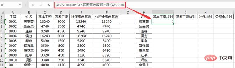
① What to look for: We need to find the employee number. The first employee number cell is A2. At the same time, in order to prevent the formula from changing when the formula is pulled to the right and filled in, an absolute reference needs to be added to lock column A, so it is $A2
② Where to search: We need to search for basic salary, provident fund, etc. in the A:F area of last month’s data. Also, in order to prevent the right pull-down filling formula from changing, an absolute reference symbol must be added, so it is “Salary basic data last month!$” A:$F”
③ Which column is returned: The basic salary is in the third column of A:F, so enter the number 3
④ 0: means precise search
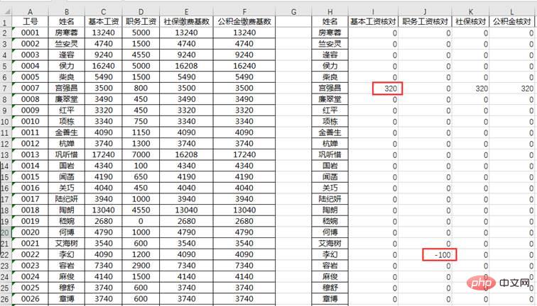
(2) Copy cell I2 and fill it into J2:L2; then modify the third parameter of the formula in J2, K2, and L2 respectively, and change it to 4, 5, and 6 in sequence; finally select I2:L2 and add it to cell L2 Double-click in the lower right corner to fill in the formula downwards to complete the data comparison. The results are as follows.
If the difference is equal to 0, it means that the data of the previous month is consistent with this month's data; if the difference is positive, it means that the data of this month has increased; if the difference is negative, it means that the data of this month has declined.
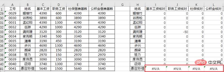
If #N/A occurs, it means that the employee's data was not found in the previous month's data table, which means that the employee is a new employee this month.
How about it? Isn't it very simple? We completed the comparison of four columns of data through a formula. Hurry up and get your hands dirty!
Related learning recommendations: excel tutorial
The above is the detailed content of Practical Excel skills sharing: Use Vlookup to compare multiple columns of data. For more information, please follow other related articles on the PHP Chinese website!

Hot AI Tools

Undresser.AI Undress
AI-powered app for creating realistic nude photos

AI Clothes Remover
Online AI tool for removing clothes from photos.

Undress AI Tool
Undress images for free

Clothoff.io
AI clothes remover

Video Face Swap
Swap faces in any video effortlessly with our completely free AI face swap tool!

Hot Article
Hot Tools

Notepad++7.3.1
Easy-to-use and free code editor

SublimeText3 Chinese version
Chinese version, very easy to use

Zend Studio 13.0.1
Powerful PHP integrated development environment

Dreamweaver CS6
Visual web development tools

SublimeText3 Mac version
God-level code editing software (SublimeText3)
Hot Topics


 What should I do if the frame line disappears when printing in Excel?
Mar 21, 2024 am 09:50 AM
What should I do if the frame line disappears when printing in Excel?
Mar 21, 2024 am 09:50 AM
If when opening a file that needs to be printed, we will find that the table frame line has disappeared for some reason in the print preview. When encountering such a situation, we must deal with it in time. If this also appears in your print file If you have questions like this, then join the editor to learn the following course: What should I do if the frame line disappears when printing a table in Excel? 1. Open a file that needs to be printed, as shown in the figure below. 2. Select all required content areas, as shown in the figure below. 3. Right-click the mouse and select the "Format Cells" option, as shown in the figure below. 4. Click the “Border” option at the top of the window, as shown in the figure below. 5. Select the thin solid line pattern in the line style on the left, as shown in the figure below. 6. Select "Outer Border"
 How to filter more than 3 keywords at the same time in excel
Mar 21, 2024 pm 03:16 PM
How to filter more than 3 keywords at the same time in excel
Mar 21, 2024 pm 03:16 PM
Excel is often used to process data in daily office work, and it is often necessary to use the "filter" function. When we choose to perform "filtering" in Excel, we can only filter up to two conditions for the same column. So, do you know how to filter more than 3 keywords at the same time in Excel? Next, let me demonstrate it to you. The first method is to gradually add the conditions to the filter. If you want to filter out three qualifying details at the same time, you first need to filter out one of them step by step. At the beginning, you can first filter out employees with the surname "Wang" based on the conditions. Then click [OK], and then check [Add current selection to filter] in the filter results. The steps are as follows. Similarly, perform filtering separately again
 How to change excel table compatibility mode to normal mode
Mar 20, 2024 pm 08:01 PM
How to change excel table compatibility mode to normal mode
Mar 20, 2024 pm 08:01 PM
In our daily work and study, we copy Excel files from others, open them to add content or re-edit them, and then save them. Sometimes a compatibility check dialog box will appear, which is very troublesome. I don’t know Excel software. , can it be changed to normal mode? So below, the editor will bring you detailed steps to solve this problem, let us learn together. Finally, be sure to remember to save it. 1. Open a worksheet and display an additional compatibility mode in the name of the worksheet, as shown in the figure. 2. In this worksheet, after modifying the content and saving it, the dialog box of the compatibility checker always pops up. It is very troublesome to see this page, as shown in the figure. 3. Click the Office button, click Save As, and then
 How to set superscript in excel
Mar 20, 2024 pm 04:30 PM
How to set superscript in excel
Mar 20, 2024 pm 04:30 PM
When processing data, sometimes we encounter data that contains various symbols such as multiples, temperatures, etc. Do you know how to set superscripts in Excel? When we use Excel to process data, if we do not set superscripts, it will make it more troublesome to enter a lot of our data. Today, the editor will bring you the specific setting method of excel superscript. 1. First, let us open the Microsoft Office Excel document on the desktop and select the text that needs to be modified into superscript, as shown in the figure. 2. Then, right-click and select the "Format Cells" option in the menu that appears after clicking, as shown in the figure. 3. Next, in the “Format Cells” dialog box that pops up automatically
 How to use the iif function in excel
Mar 20, 2024 pm 06:10 PM
How to use the iif function in excel
Mar 20, 2024 pm 06:10 PM
Most users use Excel to process table data. In fact, Excel also has a VBA program. Apart from experts, not many users have used this function. The iif function is often used when writing in VBA. It is actually the same as if The functions of the functions are similar. Let me introduce to you the usage of the iif function. There are iif functions in SQL statements and VBA code in Excel. The iif function is similar to the IF function in the excel worksheet. It performs true and false value judgment and returns different results based on the logically calculated true and false values. IF function usage is (condition, yes, no). IF statement and IIF function in VBA. The former IF statement is a control statement that can execute different statements according to conditions. The latter
 How to type subscript in excel
Mar 20, 2024 am 11:31 AM
How to type subscript in excel
Mar 20, 2024 am 11:31 AM
eWe often use Excel to make some data tables and the like. Sometimes when entering parameter values, we need to superscript or subscript a certain number. For example, mathematical formulas are often used. So how do you type the subscript in Excel? ?Let’s take a look at the detailed steps: 1. Superscript method: 1. First, enter a3 (3 is superscript) in Excel. 2. Select the number "3", right-click and select "Format Cells". 3. Click "Superscript" and then "OK". 4. Look, the effect is like this. 2. Subscript method: 1. Similar to the superscript setting method, enter "ln310" (3 is the subscript) in the cell, select the number "3", right-click and select "Format Cells". 2. Check "Subscript" and click "OK"
 Where to set excel reading mode
Mar 21, 2024 am 08:40 AM
Where to set excel reading mode
Mar 21, 2024 am 08:40 AM
In the study of software, we are accustomed to using excel, not only because it is convenient, but also because it can meet a variety of formats needed in actual work, and excel is very flexible to use, and there is a mode that is convenient for reading. Today I brought For everyone: where to set the excel reading mode. 1. Turn on the computer, then open the Excel application and find the target data. 2. There are two ways to set the reading mode in Excel. The first one: In Excel, there are a large number of convenient processing methods distributed in the Excel layout. In the lower right corner of Excel, there is a shortcut to set the reading mode. Find the pattern of the cross mark and click it to enter the reading mode. There is a small three-dimensional mark on the right side of the cross mark.
 How to insert excel icons into PPT slides
Mar 26, 2024 pm 05:40 PM
How to insert excel icons into PPT slides
Mar 26, 2024 pm 05:40 PM
1. Open the PPT and turn the page to the page where you need to insert the excel icon. Click the Insert tab. 2. Click [Object]. 3. The following dialog box will pop up. 4. Click [Create from file] and click [Browse]. 5. Select the excel table to be inserted. 6. Click OK and the following page will pop up. 7. Check [Show as icon]. 8. Click OK.
