Tips for learning Excel functions: Use the COUNTIFS function to complete unique number statistics in 1 minute

Counting duplicates and counting non-duplications are common tasks that Excel people encounter. The functions COUNTIFS (multi-condition counting function) and COUNTIF (single-condition counting function) are wonderful. They were originally used to count the number of repetitions, but through changes, they can also be used to count the number of unique ones (removing duplicate counting). For example, what are the repeated fruits below? How many fruits are there in total? If you can't answer within 5 seconds, just buy some fruit and love yourself and watch the tutorial!

Thank you all for your likes yesterday! Today I will introduce to you how to use functions to count the number of non-repeating items.

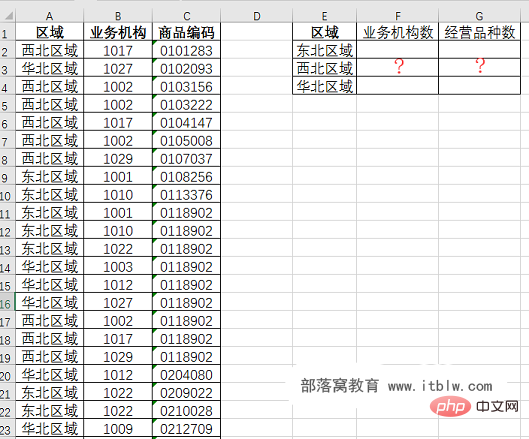
First, let’s briefly review our problem: find the number of business institutions and the number of business types in each region in the table below.

Using the new option "Add this data to the data model" in the pivot table, we can complete the above problem more easily, but there are limitations:

( 1) At least Excel Only the 2013 version will do.

(2) If you use a template for statistics, you may also need to use the vlookup function.

Isn’t there a perfect solution? there must be! Here are two function solutions shared.

The first type: COUNTIFS function with auxiliary column.

As long as we use the auxiliary column, we can get statistical results quickly using the COUNTIFS function.

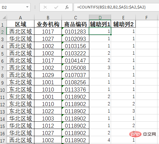
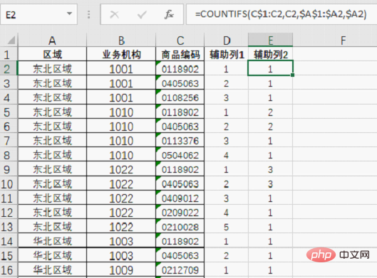
Step 1: Use the right pull-down formula to add two auxiliary columns to get the first occurrence of "1" for each business organization and the first occurrence of each product code. The formula is:

=COUNTIFS(B$1:B2,B2,$A$1:$A2,$A2)

##Explanation of formula:

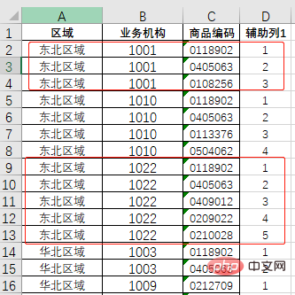
Use the first auxiliary column to illustrate the function of the formula.

In order to make it easier for everyone to view the results, the data sources are sorted by region and business organization, and the same organizations are grouped together. The result of the formula is to mark the number of times the same business organization appears in the same area in order, which is related to the next operation. Its core function is to mark the first appearance of the business organization as 1. In this way, there are as many institutions as there are 1s.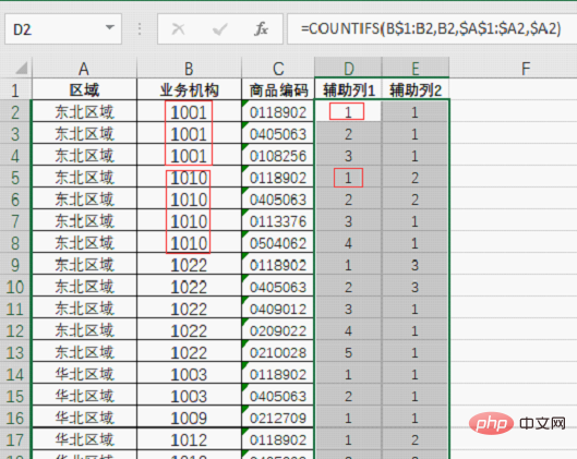

It may be the first time for some friends to use COUNTIFS. This function is very simple. It counts according to multiple conditions. The format is COUNTIFS (data area 1, condition 1, Data area 2, condition 2,...), indicating that counting will only occur if multiple conditions are met at the same time.

For example, in this example, cell D2 counts the number of times "Northeast Region (A2)" and "1001 (B2)" appear side by side in the A1:B2 area, and the result is 1 time; D4 The cell counts the number of times "Northeast Region (A4)" and "1001 (B4)" appear side by side in the area A1:B4, and the result is 3 times; the cell D9 counts the number of times "Northeast Area (A4)" and "1001 (B4)" appear side by side in the area A1:B9. Area (A9)" and "1022 (B9)", the result is 1 time...

Similarly, the second auxiliary column counts based on the region and product code. When a product appears for the first time in the same region, the result is 1:

Step 2: Enter the formula in cell H2, and then pull down right to count the number of 1's that meet the conditions in columns D and E to get the final result. The formula is: =COUNTIFS($A:$A,$G2,D:D,1)

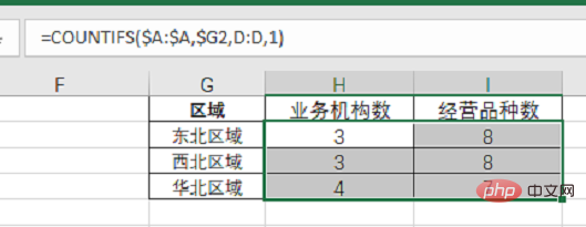
This formula is better than the auxiliary column Understand much. For example, the formula in cell H2 counts the number of times "Northeast Region" and "1" appear side by side in columns A and D.

The entire method uses only one COUNTIFS function, which is more suitable for function novices to use in memory. But for beginners, if they don’t know the role of the $ symbol in the formula, it will be difficult to understand.

A question:

If a single condition counts unique numbers, that is, the number of business institutions and the number of business types are calculated separately regardless of region, how should the formula in the above method be adjusted?

Second type: SUMPRODUCT and COUNTIFS combination formula.

The first method has auxiliary columns. Friends who like the ultimate will definitely not like it, so let’s come up with a formula that does not require auxiliary columns.

       =SUMPRODUCT(($A$2:$A$36=$G2)/COUNTIFS($A$2:$A$36,$A$2:$A$36,B$2:B$36,B $2:B$36))

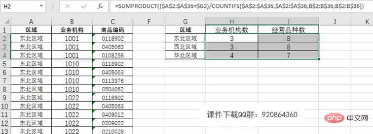
This is a relatively common "routine" formula that does not require auxiliary columns and is suitable for those who pursue the "formula to death". need. When the amount of data is not very large, it is very satisfying to complete statistics in one step.

But this formula involves a lot of array operations. When the number of rows in the data source is relatively large, it will get stuck~~~~

Another question ：

If a single condition is used to count unique numbers, that is, the number of business institutions and the number of business types are calculated separately regardless of region, how should the above formula be adjusted?

                                                                                                                                                                                                                                                                                        PI PI P PI P PL Friends are welcome to throw bricks. The more bricks you throw, the happier the newbie will be. At the same time, if you think it’s good, please don’t eat it alone and share it with your friends generously and enthusiastically

Related learning recommendations: excel tutorial

The above is the detailed content of Tips for learning Excel functions: Use the COUNTIFS function to complete unique number statistics in 1 minute. For more information, please follow other related articles on the PHP Chinese website!