Excel Chart Learning Super Simple Dynamic Chart Tutorial (Getting Started)

The author combines teaching with learning, and makes the boring excel tutorial feel like a martial arts competition. I believe many novel fans will go crazy for it! This tutorial is an introduction to dynamic charts. The knowledge points are not difficult, but they are very useful in work. Just treat this tutorial as if you are reading a martial arts novel!

The sun and the moon reincarnate, and the stars change. In the world, the new generation of martial arts leaders are tired of the turmoil of the world and intend to retire. However, they have not been able to find a highly respected successor, so they have ordered that within one year, who can be just? The person who kills demons and teaches the most people will take over as the new leader of the martial arts alliance. From then on, murderous plots arose in the martial arts world, and the world was full of bloodshed.

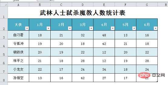
It was past half time. One day in the main hall, spies came to report: Alliance Leader, in the past six months, heroes from all walks of life have fought bravely to kill the enemy, which has frightened the followers of the Demon Cult and caused more than half of them to be killed or injured. These are the top 6 heroes killed. number of enemies.

The leader took over the iPad and saw an excel sheet. He was very happy and proud.

But in an instant, his expression changed from joy to anger, and he was furious: How come your excel level is so bad? It is not even one-tenth of the skill of the demon sect. If this continues, Taiping Jianghu will eventually be destroyed. Hands, hoohoo, it hurts, it's sad...

Everyone felt ashamed, but they didn't dare to say a word. The leader was helpless and projected on the spot to demonstrate: "Although you have tried your best to help take care of the matter, it's more important than ever." All the original data analysis needs to be done in my hands. This is not an efficient approach. I will give you an example, hoping that it will have the effect of inspiring others. The following GIF effects are the minimum standards we pursue.

As the saying goes: If you practice qi without practicing qigong, you will be in vain; if you practice qigong without practicing qi, your efforts will be in vain. The way to practice excel is divided into internal skills and external skills. Today, I will lead you to the introductory chapter of practicing internal skills and mental methods - the simplest effect creation of dynamic charts.

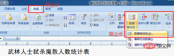
The first type of dynamic chart: making a drop-down menu

The first type is essentially the content of external training, so internal training must have Only with a certain foundation of external skills training and the combination of internal and external skills can you develop superior skills.

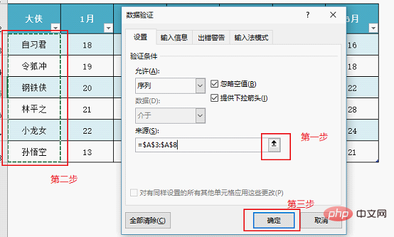
The creation of the drop-down menu is very simple. Click on cell A10 to bring up the data verification dialog box. Just enter all items under Data Verification—Sequence—Source, and end it with a comma ( English status) can be separated, as shown below.

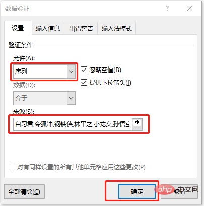
#Of course, if there is a lot of drop-down data, inputting like this is very troublesome and easy to make mistakes. Is there a better way? We can click to select the data source at Data Validation - Source.

The second method of dynamic chart: refer to the data source

The functions to be achieved by this method are: When a hero is selected from the drop-down menu, the subsequent cells automatically display the data corresponding to the hero from January to June. There are many ways to implement this function, the most commonly used is to directly use the vertical lookup function VLOOKUP to return.

VLOOKUP (Who to look for? Where to look for? Which column value is returned? Exact OR fuzzy search?)

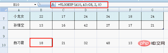
In unit The formula entered in box B10 is: =VLOOKUP(A10,A3:G8,2,0)

Formula analysis:

is expressed in A3 : The first column of the G8 area, search for the content of A10 (i.e. "self-study gentleman"), if "self-study gentleman" is found, return A3: the data of the second column of the G8 area (i.e. "18"), if not found, return an error (i.e. "#N/A"). In cells C10-G10, change the third parameter to 3, 4, 5...

Of course, if you have mastered the inner strength and mental skills, you can directly enter = in cells B10 to G10. VLOOKUP($A$10,$A$3:$G$8,COLUMN(),0) is enough. The value returned by the COLUMN() function is the number of columns corresponding to the cell where it is located.

In the future practice, you will find many such flexible operation methods. Practice has proved that the more you practice the Excel Dafa, the more flexible it becomes. All roads lead to Rome, until there is no way to win but there is always a way to win.

The third type of dynamic chart: Insert chart

Press the Ctrl key and select the cells in row 2 and row 10 in sequence. Insert a column chart.

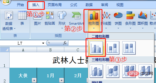
The charts automatically generated after insertion are as follows:

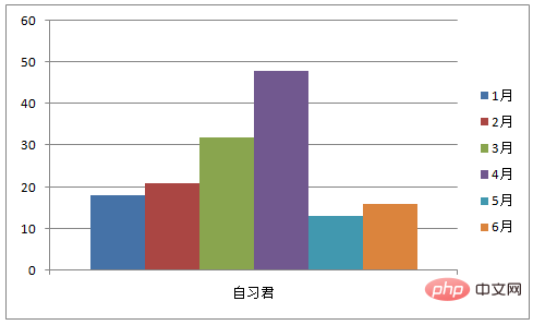
When people practice, there are few people who study charts. The reason is: The reason is that there are fewer opportunities for practical application, and it is a function that is icing on the cake; the second reason is that the effect of improving work efficiency is not obvious, and success in practice is not something that can be accomplished in a day. But in many cases, charts are an intuitive reflection of data processing. Compared with cold cells, charts can have the effect of "one table" and "silence is better than sound".

The fourth type of dynamic chart: beautify the chart

In fact, the charts automatically generated by each version of excel look different, but they all have the same appearance. One characteristic: ugly... I am a Virgo, and it is really unbearable for messy layouts, tables with non-uniform formats, and unbeautified charts. Now Lao Na uses the sword technique of "the flowers gradually become charming" to beautify and beautify everyone.

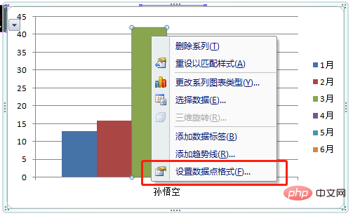
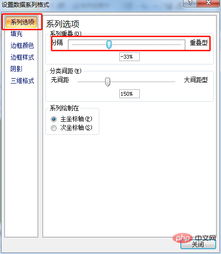
Step one: Adjust the width of the column chart. Right-click the column chart and set the format of the data series - separate overlapping series.

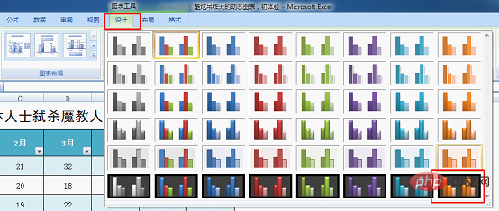
Step 2: Apply the format. Set the chart style - select black shading (I like the dark night, and the dark night makes me look forward to the brighter light).

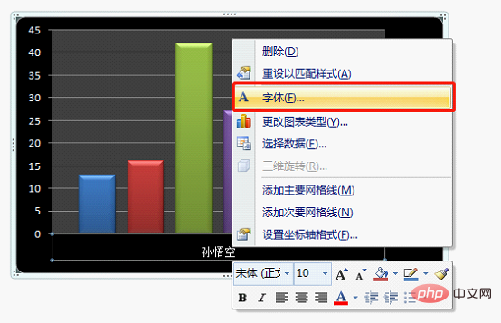
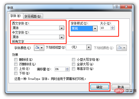
Step 3: Adjust the font size. Right-click on the text and set the font format.

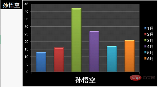
The final effect is as follows:

Lao Na just had a whim today. The martial arts leader solves problems. As the saying goes, "If you want to practice this skill, you must first practice self-control." In fact, in the eyes of experts, the above cultivation method is extremely stupid and is a manifestation of self-control. I now have a practice that "can be successful even without self-control" The method only needs to be operated with the mouse for more than ten seconds. To predict the future events, please see the next chapter for details.

Related learning recommendations: excel tutorial

The above is the detailed content of Excel Chart Learning Super Simple Dynamic Chart Tutorial (Getting Started). For more information, please follow other related articles on the PHP Chinese website!