Excel case sharing: 5 efficient techniques that can be achieved by just 'drag and drag'

In the previous article "Excel Case Sharing: Calculation Methods for Year-on-Year Growth Rate and Month-on-Month Growth in Each Year", we learned the calculation methods for year-on-year growth rate and month-on-month growth in each year. Today we are going to talk about 5 commonly used skills in Excel tables. Unexpectedly, the problem that has troubled me for a long time can be solved with just drag and drop shortcut keys. To be honest, you think function charts are too difficult to learn, but today you must learn these few tips to solve problems by just dragging with the mouse!

#Someone once said that Excel is inseparable from the mouse, and the real masters are all keyboardists! Xiaohua doesn’t think so. The so-called master is one who can give full play to the role of various tools, and there is always a trick to win! If you don’t believe it, let’s take a look at the efficient “drag and drag” skills in Excel. These are all Excel table office skills.

part 1 Excel dragging and hiding skills

skill 1, after selecting multiple rows, drag to adjust any row Or the row width or column width of a column, then all selected rows or columns will be batch adjusted to the same row height/column width.

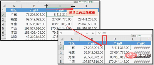
skill 2, drag a row edge upward or drag a column edge left until the two edges of the row/column overlap, that is This row/column can be hidden. Continue dragging the edge up or to the left to hide multiple rows/columns.

skill 3, for rows or columns that have been hidden or excluded by filtering, we can also drag the edges to make these hidden rows and columns " Show up”!

For example, the third row in the picture below is hidden (in the picture, it is filtered and hidden, it may be hidden by email, or it may be hidden by dragging as we just talked about).

At this time, move the mouse to the edge of the hidden row (column) (the image below indicates the location), and wait until the mouse turns into a double-line double-arrow cross (the column title is ), hold down the left mouse button and drag the edge downward (or right), and release the mouse to unhide the row/column.

part 2 Excel right-click dragging skills

Right-click dragging of the mouse, this is a link to Excel Skills that even veterans don’t know. Its functions are very down-to-earth. One mouse can handle those frequently used small actions.

1. Select a continuous data range. Move the mouse to the right edge of the area, and the mouse will change into a solid arrow cross;

2. Hold down the right mouse button and drag the area to any location.

#3. Release the mouse, the right-click drag menu will pop up, and select the corresponding function.

The right-click menu can complete multiple functions such as inserting, copying, and linking. Below we will only demonstrate a special usage, which can remove the formula and only retain the numerical value.

Select the continuous cell range, hold down the right mouse button and drag in any direction and then drag it back to the original position (be careful not to release the right mouse button during the process), select [Copy Value Only], and done!

part 3 shift key - insert and move skills

skill 1 insert blank Rows/Empty Columns

How do you insert empty rows/columns? Use the right-click menu - Insert, or select the corresponding function in the [Start] tab - [Insert]. Congratulations, you will soon learn the third more convenient way, which is Shift key and left mouse button dragging to insert.

step 1 Select a row or column, move the mouse to the small solid square at the bottom right of the row header or column header, the mouse will turn into a black cross, hold down the Shift key, and the mouse will turn into Double line double arrow cross;

step 2 Keep pressing the Shift key and hold down the left mouse button at the same time, drag down or to the right to make the lower or right edge of the selected row/column overlap with the edges of other rows or columns;

#step 3 Release the left mouse button and drag the row/column edge as many rows/columns as you want to insert the corresponding number of rows/rows below or to the right of the selected row. Column

skill 2 Move the area to the specified position

Shift key and left-click dragging can insert the cell range to the specified location (current worksheet only).

step 1 Select a continuous cell range, move the mouse to the edge of the range, and the mouse turns into a solid cross with an arrow;

Step 2 Press Hold down the Shift key, press the left mouse button at the same time, and drag the mouse to the specified position. At this time, the edge of the specified position changes to a highlighted line segment, indicating that it is inserted below the line. If you drag a column, the vertical line that appears is inserted to the right of the line.

#Step 3 Release the mouse and keyboard to complete the movement of the cell area.

What’s even more special is that if we choose to Shift-drag a row or column into an adjacent row/column position, we can achieve the so-called “exchange rows/columns” ".

step 1 Click the row/column title, select the row/column, and move the mouse to the row/column edge. Hold down the Shift key and the left mouse button at the same time, and drag the row/column to the edge of the adjacent row/column.

#step 2 Release Shift and the left mouse button to complete the row/column exchange.

part 4 Ctrl key-drag copy skills

skill 1 Drag Copy the cell area

Step 1 Select the cell area, move the mouse to the edge of the cell area, the mouse will change into a solid cross with an arrow, hold down the Ctrl key, and black will appear above the mouse graphic Cross symbol. Press and hold the left mouse button at the same time and drag the selected area to the specified location.

#step 2 Release the mouse to complete the copy.

#Ctrl dragging method can not only copy the cell range, but also copy the worksheet.

Skill 2 Copy the worksheet

step 1 Move the mouse to the worksheet label, hold down the Ctrl key and the left mouse button at the same time, and drag in any direction. At this point the mouse changes to .

step 2 After dragging the mouse to any position, release the mouse to complete the copy. Note that during the dragging process, a solid black inverted triangle will appear above the worksheet label, indicating that the worksheet will be copied behind the triangle.

part 5 Alt key - cross-table copy skills

If the petals want to achieve cross-table replication To copy a cell range, you need to know the third key related to dragging, which is the Alt key.

Still familiar method, still the same operation! No need to go into details here, just go to the picture!

If you are smart, you may have discovered that Ctrl, Shift and Alt seem to be able to be parallelized, that is, copy, insert, cross-table copy, etc. If you are smarter, you may also find that these three shortcut keys also have a different style when used for dragging. If Xiaohua’s article makes you eager to try it, you might as well open your Excel and review all the dragging skills you know. If you have any new discoveries or new uses, please leave a message to share!

Related learning recommendations: excel tutorial

The above is the detailed content of Excel case sharing: 5 efficient techniques that can be achieved by just 'drag and drag'. For more information, please follow other related articles on the PHP Chinese website!