

Example summary of eight uses of the AGGREGATE function in Excel

This article brings you relevant knowledge about excel, which mainly introduces the relevant content about the AGGREGATE function. The usage of this function is similar to the SUBTOTAL function, but it is more functional than the SUBTOTAL function. It's powerful, let's take a look at it, I hope it will be helpful to everyone.
Related learning recommendations: excel tutorial
The usage of the AGGREGATE function is similar to the SUBTOTAL function, but it is more powerful than the SUBTOTAL function. , not only can realize the functions of 19 functions such as SUM, AVERAGE, COUNT, LARGE, MAX, etc., but also can ignore hidden rows, error values, null values, etc., and supports constant arrays.
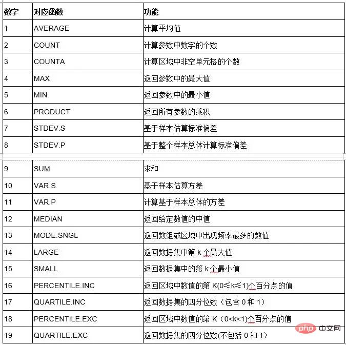
The first parameter of this function is a number between 1 and 19, used to specify the summary method to be used:
The second parameter is the A number between 0 and 7, specifying which types of values to ignore in the calculation area:

Next let’s talk about some typical uses of this function:
1. Multiple discontinuous areas ignore error values and directly sum them
The power of this function is that the 2nd parameter can be specified to ignore error values and directly count
As follows Figure, the blue area contains different error values, now we need to sum these discontinuous areas.
The formula is:
=AGGREGATE(9,6,A3:A7,C3:C4,D6:F7)

2. Ignore error values in filtering state
As shown below, the filtered data area contains error values. How to count the visible cells?
The formula is:
=AGGREGATE(9,7,B6:B18)

=AGGREGATE({4;5;1;9;3;12},{5,0},B4:B14)

=AGGREGATE(9,3,A4:A$18)*2-AGGREGATE(9,7,A4:A$18)
=AGGREGATE(15,6,B4:B15/(A4:A15="1 workshop" ),1)

=IFERROR(INDEX(B:B,AGGREGATE(15,6,ROW( $3:$12)/(A$3:A$12=D$3),ROW(A1))),"")

The idea of this formula is basically the same as the fifth formula.
7. Count the maximum value in the same cell
As shown below, the assessment status of multiple people in column B is written in the same cell, and the maximum value must be counted. The formula is:
=AGGREGATE(14,6,--MID(B4,ROW($1:$50),COLUMN(A:AZ)),1)

For the MID(B4,ROW($1:$50),COLUMN(A:AZ)) part of the formula, use the MID function, starting from the 1st to 50th characters, and extract each A string with a length of 1~50 will result in a huge memory array. Use two more negative signs to turn the text in the memory array into an error value, and the value is still its own value.
Finally use the AGGREGATE function to ignore the error values in the memory array and calculate the first minimum value among them.
8. Simultaneously count the maximum and minimum values of the specified conditions
As shown in the figure below, it is necessary to count the maximum and minimum values corresponding to 1 workshop at the same time.
First select cells F4:G4 at the same time, enter the following formula in the edit bar, press Ctrl Shift and press Enter.
=AGGREGATE({16,15},6,B4:B15/(A4:A15=E4),1)

AGGREGATE The first parameter uses the constant array {16,15}, which indicates the calculation rules of using the maximum value and the minimum value respectively.
The final result is also a memory array, so two cells must be selected for input at the same time.
The characteristic of this function is that when the first parameter is 14~19, you can use the fourth parameter. At this time, the fourth parameter supports arrays, so you can play various applications to replace the direct SMALL, LARGE and other functions that ignore error values.
Related learning recommendations: excel tutorial
The above is the detailed content of Example summary of eight uses of the AGGREGATE function in Excel. For more information, please follow other related articles on the PHP Chinese website!

Hot AI Tools

Undresser.AI Undress
AI-powered app for creating realistic nude photos

AI Clothes Remover
Online AI tool for removing clothes from photos.

Undress AI Tool
Undress images for free

Clothoff.io
AI clothes remover

Video Face Swap
Swap faces in any video effortlessly with our completely free AI face swap tool!

Hot Article
Hot Tools

Notepad++7.3.1
Easy-to-use and free code editor

SublimeText3 Chinese version
Chinese version, very easy to use

Zend Studio 13.0.1
Powerful PHP integrated development environment

Dreamweaver CS6
Visual web development tools

SublimeText3 Mac version
God-level code editing software (SublimeText3)
Hot Topics
 1671
1671
 14
1428
52
1329
25
1276
29
1256
24
14
1428
52
1329
25
1276
29
1256
24

 What should I do if the frame line disappears when printing in Excel?
Mar 21, 2024 am 09:50 AM
What should I do if the frame line disappears when printing in Excel?
Mar 21, 2024 am 09:50 AM
If when opening a file that needs to be printed, we will find that the table frame line has disappeared for some reason in the print preview. When encountering such a situation, we must deal with it in time. If this also appears in your print file If you have questions like this, then join the editor to learn the following course: What should I do if the frame line disappears when printing a table in Excel? 1. Open a file that needs to be printed, as shown in the figure below. 2. Select all required content areas, as shown in the figure below. 3. Right-click the mouse and select the "Format Cells" option, as shown in the figure below. 4. Click the “Border” option at the top of the window, as shown in the figure below. 5. Select the thin solid line pattern in the line style on the left, as shown in the figure below. 6. Select "Outer Border"
 How to filter more than 3 keywords at the same time in excel
Mar 21, 2024 pm 03:16 PM
How to filter more than 3 keywords at the same time in excel
Mar 21, 2024 pm 03:16 PM
Excel is often used to process data in daily office work, and it is often necessary to use the "filter" function. When we choose to perform "filtering" in Excel, we can only filter up to two conditions for the same column. So, do you know how to filter more than 3 keywords at the same time in Excel? Next, let me demonstrate it to you. The first method is to gradually add the conditions to the filter. If you want to filter out three qualifying details at the same time, you first need to filter out one of them step by step. At the beginning, you can first filter out employees with the surname "Wang" based on the conditions. Then click [OK], and then check [Add current selection to filter] in the filter results. The steps are as follows. Similarly, perform filtering separately again
 How to change excel table compatibility mode to normal mode
Mar 20, 2024 pm 08:01 PM
How to change excel table compatibility mode to normal mode
Mar 20, 2024 pm 08:01 PM
In our daily work and study, we copy Excel files from others, open them to add content or re-edit them, and then save them. Sometimes a compatibility check dialog box will appear, which is very troublesome. I don’t know Excel software. , can it be changed to normal mode? So below, the editor will bring you detailed steps to solve this problem, let us learn together. Finally, be sure to remember to save it. 1. Open a worksheet and display an additional compatibility mode in the name of the worksheet, as shown in the figure. 2. In this worksheet, after modifying the content and saving it, the dialog box of the compatibility checker always pops up. It is very troublesome to see this page, as shown in the figure. 3. Click the Office button, click Save As, and then
 How to type subscript in excel
Mar 20, 2024 am 11:31 AM
How to type subscript in excel
Mar 20, 2024 am 11:31 AM
eWe often use Excel to make some data tables and the like. Sometimes when entering parameter values, we need to superscript or subscript a certain number. For example, mathematical formulas are often used. So how do you type the subscript in Excel? ?Let’s take a look at the detailed steps: 1. Superscript method: 1. First, enter a3 (3 is superscript) in Excel. 2. Select the number "3", right-click and select "Format Cells". 3. Click "Superscript" and then "OK". 4. Look, the effect is like this. 2. Subscript method: 1. Similar to the superscript setting method, enter "ln310" (3 is the subscript) in the cell, select the number "3", right-click and select "Format Cells". 2. Check "Subscript" and click "OK"
 How to set superscript in excel
Mar 20, 2024 pm 04:30 PM
How to set superscript in excel
Mar 20, 2024 pm 04:30 PM
When processing data, sometimes we encounter data that contains various symbols such as multiples, temperatures, etc. Do you know how to set superscripts in Excel? When we use Excel to process data, if we do not set superscripts, it will make it more troublesome to enter a lot of our data. Today, the editor will bring you the specific setting method of excel superscript. 1. First, let us open the Microsoft Office Excel document on the desktop and select the text that needs to be modified into superscript, as shown in the figure. 2. Then, right-click and select the "Format Cells" option in the menu that appears after clicking, as shown in the figure. 3. Next, in the “Format Cells” dialog box that pops up automatically
 How to use the iif function in excel
Mar 20, 2024 pm 06:10 PM
How to use the iif function in excel
Mar 20, 2024 pm 06:10 PM
Most users use Excel to process table data. In fact, Excel also has a VBA program. Apart from experts, not many users have used this function. The iif function is often used when writing in VBA. It is actually the same as if The functions of the functions are similar. Let me introduce to you the usage of the iif function. There are iif functions in SQL statements and VBA code in Excel. The iif function is similar to the IF function in the excel worksheet. It performs true and false value judgment and returns different results based on the logically calculated true and false values. IF function usage is (condition, yes, no). IF statement and IIF function in VBA. The former IF statement is a control statement that can execute different statements according to conditions. The latter
 Where to set excel reading mode
Mar 21, 2024 am 08:40 AM
Where to set excel reading mode
Mar 21, 2024 am 08:40 AM
In the study of software, we are accustomed to using excel, not only because it is convenient, but also because it can meet a variety of formats needed in actual work, and excel is very flexible to use, and there is a mode that is convenient for reading. Today I brought For everyone: where to set the excel reading mode. 1. Turn on the computer, then open the Excel application and find the target data. 2. There are two ways to set the reading mode in Excel. The first one: In Excel, there are a large number of convenient processing methods distributed in the Excel layout. In the lower right corner of Excel, there is a shortcut to set the reading mode. Find the pattern of the cross mark and click it to enter the reading mode. There is a small three-dimensional mark on the right side of the cross mark.
 How to insert excel icons into PPT slides
Mar 26, 2024 pm 05:40 PM
How to insert excel icons into PPT slides
Mar 26, 2024 pm 05:40 PM
1. Open the PPT and turn the page to the page where you need to insert the excel icon. Click the Insert tab. 2. Click [Object]. 3. The following dialog box will pop up. 4. Click [Create from file] and click [Browse]. 5. Select the excel table to be inserted. 6. Click OK and the following page will pop up. 7. Check [Show as icon]. 8. Click OK.
