

How to split cell content

How to split the cell content: first select the cell, enter the data column, and click the column option; then check the delimiter symbol, click Next; finally check the space and general options, and click Finish. .

The operating environment of this article: windows10 system, microsoft office excel 2010, thinkpad t480 computer.
The specific method is as follows:
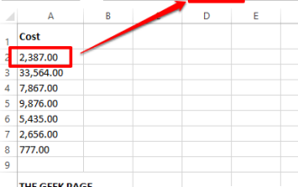
First we enter some data in the excel table. For example, I enter the name and scores here, separated by the space bar.

Select the data-click data options-select columns.

In the Text Splitting Wizard 1, select the delimiter and next step.

In the Text Sorting Wizard 2, check the box and click next.

In the Text Splitting Wizard 3, select General and click Finish.

Looking at the final effect, I found that one cell has been divided into two cells.

Related recommendations: excel basic tutorial
The above is the detailed content of How to split cell content. For more information, please follow other related articles on the PHP Chinese website!

Hot AI Tools

Undresser.AI Undress
AI-powered app for creating realistic nude photos

AI Clothes Remover
Online AI tool for removing clothes from photos.

Undress AI Tool
Undress images for free

Clothoff.io
AI clothes remover

Video Face Swap
Swap faces in any video effortlessly with our completely free AI face swap tool!

Hot Article
Hot Tools

Notepad++7.3.1
Easy-to-use and free code editor

SublimeText3 Chinese version
Chinese version, very easy to use

Zend Studio 13.0.1
Powerful PHP integrated development environment

Dreamweaver CS6
Visual web development tools

SublimeText3 Mac version
God-level code editing software (SublimeText3)
Hot Topics


 Excel found a problem with one or more formula references: How to fix it
Apr 17, 2023 pm 06:58 PM
Excel found a problem with one or more formula references: How to fix it
Apr 17, 2023 pm 06:58 PM
Use an Error Checking Tool One of the quickest ways to find errors with your Excel spreadsheet is to use an error checking tool. If the tool finds any errors, you can correct them and try saving the file again. However, the tool may not find all types of errors. If the error checking tool doesn't find any errors or fixing them doesn't solve the problem, then you need to try one of the other fixes below. To use the error checking tool in Excel: select the Formulas tab. Click the Error Checking tool. When an error is found, information about the cause of the error will appear in the tool. If it's not needed, fix the error or delete the formula causing the problem. In the Error Checking Tool, click Next to view the next error and repeat the process. When not
 How to set the print area in Google Sheets?
May 08, 2023 pm 01:28 PM
How to set the print area in Google Sheets?
May 08, 2023 pm 01:28 PM
How to Set GoogleSheets Print Area in Print Preview Google Sheets allows you to print spreadsheets with three different print areas. You can choose to print the entire spreadsheet, including each individual worksheet you create. Alternatively, you can choose to print a single worksheet. Finally, you can only print a portion of the cells you select. This is the smallest print area you can create since you could theoretically select individual cells for printing. The easiest way to set it up is to use the built-in Google Sheets print preview menu. You can view this content using Google Sheets in a web browser on your PC, Mac, or Chromebook. To set up Google
 How to embed a PDF document in an Excel worksheet
May 28, 2023 am 09:17 AM
How to embed a PDF document in an Excel worksheet
May 28, 2023 am 09:17 AM
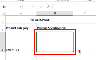
It is usually necessary to insert PDF documents into Excel worksheets. Just like a company's project list, we can instantly append text and character data to Excel cells. But what if you want to attach the solution design for a specific project to its corresponding data row? Well, people often stop and think. Sometimes thinking doesn't work either because the solution isn't simple. Dig deeper into this article to learn how to easily insert multiple PDF documents into an Excel worksheet, along with very specific rows of data. Example Scenario In the example shown in this article, we have a column called ProductCategory that lists a project name in each cell. Another column ProductSpeci
 How to create a random number generator in Excel
Apr 14, 2023 am 09:46 AM
How to create a random number generator in Excel
Apr 14, 2023 am 09:46 AM
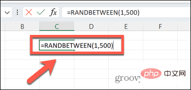
How to use RANDBETWEEN to generate random numbers in Excel If you want to generate random numbers within a specific range, the RANDBETWEEN function is a quick and easy way to do it. This allows you to generate random integers between any two values of your choice. Generate random numbers in Excel using RANDBETWEEN: Click the cell where you want the first random number to appear. Type =RANDBETWEEN(1,500) replacing "1" with the lowest random number you want to generate and "500" with
 How to remove commas from numeric and text values in Excel
Apr 17, 2023 pm 09:01 PM
How to remove commas from numeric and text values in Excel
Apr 17, 2023 pm 09:01 PM
On numeric values, on text strings, using commas in the wrong places can really get annoying, even for the biggest Excel geeks. You may even know how to get rid of commas, but the method you know may be time-consuming for you. Well, no matter what your problem is, if it is related to a comma in the wrong place in your Excel worksheet, we can tell you one thing, all your problems will be solved today, right here! Dig deeper into this article to learn how to easily remove commas from numbers and text values in the simplest steps possible. Hope you enjoy reading. Oh, and don’t forget to tell us which method catches your eye the most! Section 1: How to Remove Commas from Numerical Values When a numerical value contains a comma, there are two possible situations:
 How to enable Sensitive Content Warning on iPhone and learn about its features
Sep 22, 2023 pm 12:41 PM
How to enable Sensitive Content Warning on iPhone and learn about its features
Sep 22, 2023 pm 12:41 PM
Especially over the past decade, mobile devices have become the primary way to share content with friends and family. The easy-to-access, easy-to-use interface and ability to capture images and videos in real time make it a great choice for creating and sharing content. However, it's easy for malicious users to abuse these tools to forward unwanted, sensitive content that may not be suitable for viewing and does not require your consent. To prevent this from happening, a new feature with "Sensitive Content Warning" was introduced in iOS17. Let's take a look at it and how to use it on your iPhone. What is the new Sensitive Content Warning and how does it work? As mentioned above, Sensitive Content Warning is a new privacy and security feature designed to help prevent users from viewing sensitive content, including iPhone
 How to find and delete merged cells in Excel
Apr 20, 2023 pm 11:52 PM
How to find and delete merged cells in Excel
Apr 20, 2023 pm 11:52 PM
How to Find Merged Cells in Excel on Windows Before you can delete merged cells from your data, you need to find them all. It's easy to do this using Excel's Find and Replace tool. Find merged cells in Excel: Highlight the cells where you want to find merged cells. To select all cells, click in an empty space in the upper left corner of the spreadsheet or press Ctrl+A. Click the Home tab. Click the Find and Select icon. Select Find. Click the Options button. At the end of the FindWhat settings, click Format. Under the Alignment tab, click Merge Cells. It should contain a check mark rather than a line. Click OK to confirm the format
 How to use the SIGN function in Excel to determine the sign of a value
May 07, 2023 pm 10:37 PM
How to use the SIGN function in Excel to determine the sign of a value
May 07, 2023 pm 10:37 PM
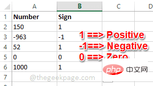
The SIGN function is a very useful function built into Microsoft Excel. Using this function you can find out the sign of a number. That is, whether the number is positive. The SIGN function returns 1 if the number is positive, -1 if the number is negative, and zero if the number is zero. Although this sounds too obvious, if you have a large column containing many numbers and we want to find the sign of all the numbers, it is very useful to use the SIGN function and get the job done in a few seconds. In this article, we explain 3 different methods on how to easily use the SIGN function in any Excel document to calculate the sign of a number. Read on to learn how to master this cool trick. start up
