

What is breadth-first traversal of a graph similar to a binary tree?

Breadth-first traversal of a graph is horizontal-first traversal, similar to layer-by-layer traversal of a binary tree. Breadth-first traversal searches and traverses along the width of the tree starting from the root node, that is, traversing in a hierarchical manner; each layer is visited sequentially from top to bottom, and in each layer, from left to right (or right to left) To access nodes, after accessing one level, enter the next level until no nodes can be accessed.

1. Introduction
Similar to tree traversal, graph traversal also starts from a certain point in the graph, and then traverses it according to a certain method. All vertices in the graph are visited only once.
But graph traversal is more complicated than trees. Because any vertex in the graph may be adjacent to other vertices, the visited vertices must be recorded during graph traversal to avoid repeated visits.
According to different search paths, we can divide the methods of graph traversal into two types: breadth-first search and depth-first search.
2. Basic concepts of graphs
2.1. Undirected graphs and undirected graphs
The vertex pair (u, v) is unordered, that is, (u, v ) and (v, u) are the same side. Usually expressed by a pair of parentheses.
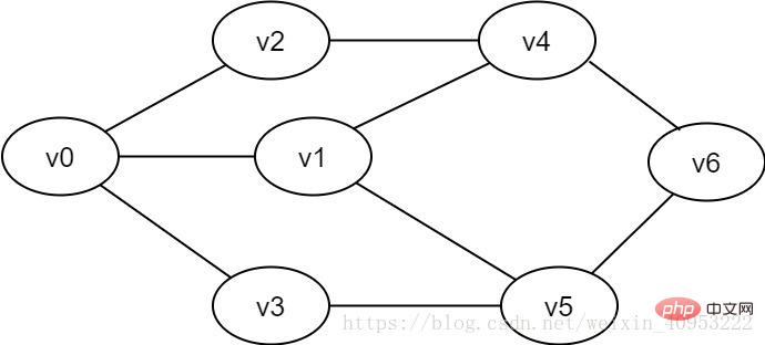
Figure 2-1-1 Example of an undirected graph
The vertex pair
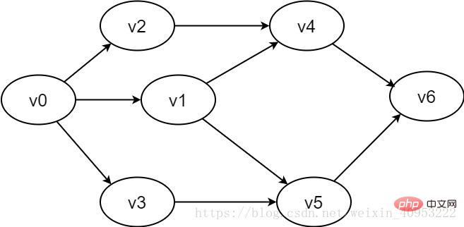
Figure 2-1-2 Example of a directed graph
##2.2 .Quanhe.net
Each edge of the graph may have a value with a certain meaning, which is called the weight of the edge. This kind of weighted graph is called a network. 2.3. Connected graphs and non-connected graphsConnected graph: In the undirected graph G, if there is a path from vertex v to vertex v', then v and v' are said to be connected. If any two vertices v, v'∈V in the graph, and v and v' are connected, then G is said to be a connected graph. The above two graphs are both connected graphs. Disconnected graph: If there is a disconnection between v and v' in the undirected graph G, then G is said to be a disconnected graph.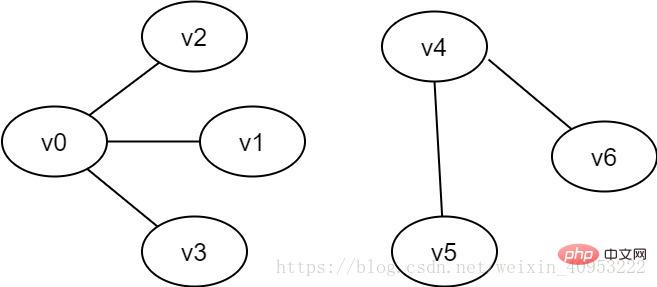
Figure 2-3 Example of a non-connected graph
3. Breadth-first search
3.1. Basic idea of the algorithmBreadth-first search is similar to the hierarchical traversal process of a tree. It needs to be implemented with the help of a queue. As shown in Figure 2-1-1, if we want to traverse every vertex from v0 to v6, we can set v0 as the first layer, v1, v2, and v3 as the second layer, v4 and v5 as the third layer, and v6 For the fourth layer, each vertex of each layer is traversed one by one. The specific process is as follows: 1. Preparation: Create a visited array to record the visited vertices; create a queue to store the vertices of each layer; initialization Figure G. 2. Start visiting from v0 in the figure, set the value of the visited[v0] array to true, and add v0 to the queue. 3. As long as the queue is not empty, repeat the following operations: (1) Point u at the head of the team to exit the queue. (2) Check all adjacent vertices w of u in turn. If the value of visited[w] is false, visit w, set visited[w] to true, and add w to the queue. 3.2. Implementation process of the algorithmWhite means it has not been visited, gray means it is about to be visited, and black means it has been visited.
visited array: 0 means not visited, 1 means visited.
Queue: elements come out from the head of the queue and elements enter from the tail.
1. Initially, all vertices have not been visited, the visited array is initialized to 0, and there are no elements in the queue.
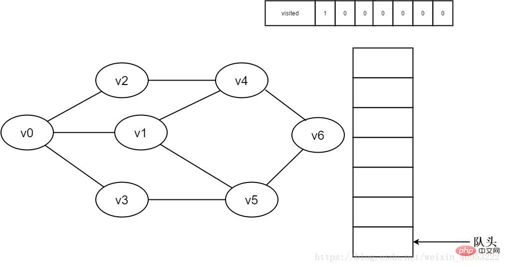
Figure 3-2-1
#2. Vertex v0 is about to be visited.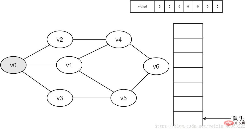
Figure 3-2-2
3. Visit vertex v0 and place visited[0 The value of ] is 1, and v0 is added to the queue at the same time.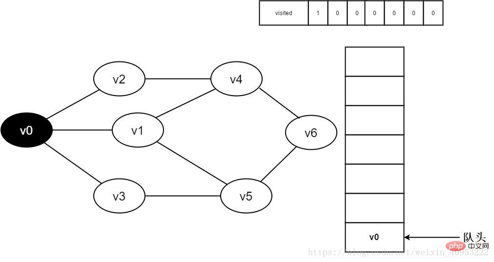
Figure 3-2-3
4. Dequeue v0 and visit v0’s adjacent point v2. Determine visited[2], because the value of visited[2] is 0, visit v2.
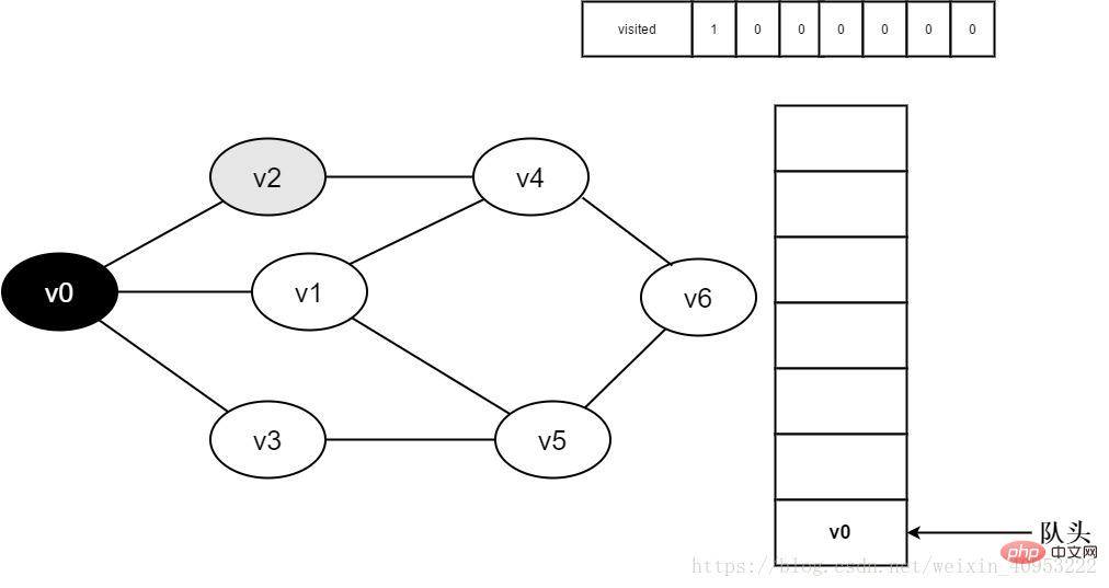
Figure 3-2-4
5. Set visited[2] to 1 and v2 Join the team.

Figure 3-2-5
6. Access v0 neighbor point v1. Determine visited[1], because the value of visited[1] is 0, visit v1.
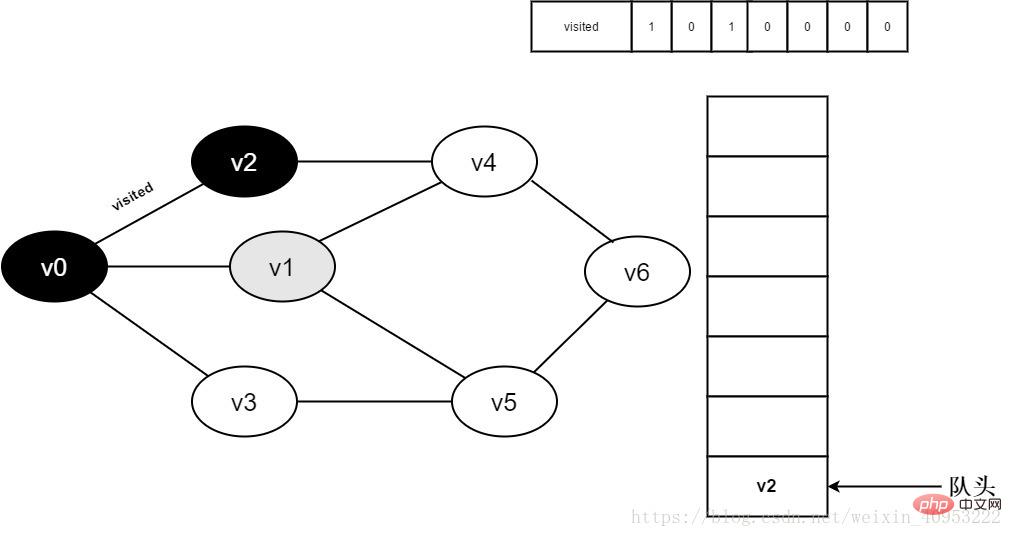
Figure 3-2-6
7. Set visited[1] to 0 and v1 Join the team.
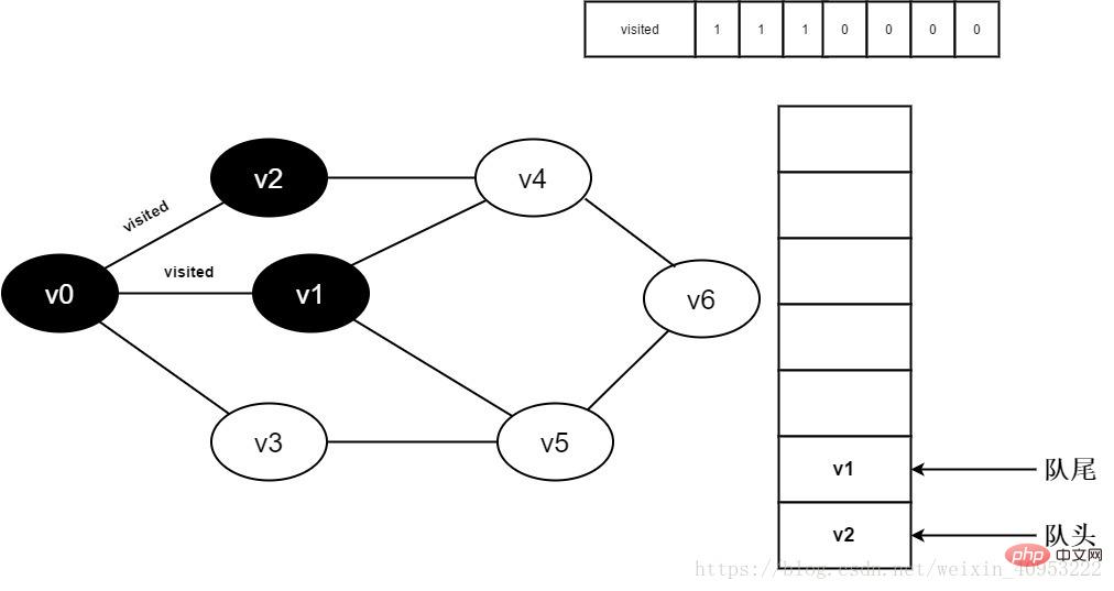
Figure 3-2-7
8. Judge visited[3] because its value is 0 , access v3. Set visited[3] to 0 and enqueue v3.
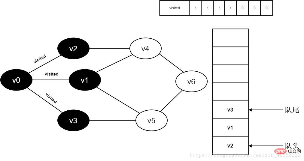
All adjacent points of Figure 3-2-8
9.v0 have been visited. Dequeue the head element v2 and start visiting all adjacent points of v2.
Start visiting v2 adjacent point v0, and judge visited[0]. Because its value is 1, no visit will be performed.
Continue to visit v2 adjacent point v4, judge visited[4], because its value is 0, visit v4, as shown below:
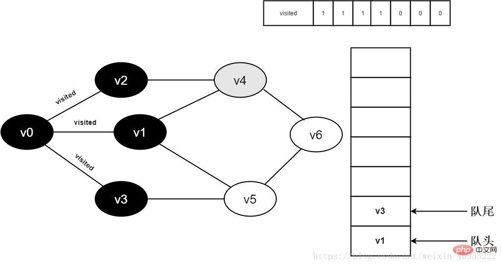
Figure 3-2-9
10. Set visited[4] to 1 and add v4 to the queue.

Figure 3-2-10
All adjacent points of 11.v2 have been visited. Dequeue the head element v1 and start visiting all adjacent points of v1.
Start visiting v1 adjacent point v0, because the visited[0] value is 1, no visit is performed.
Continue to visit v1 adjacent point v4, because the value of visited[4] is 1, no visit is performed.
Continue to visit v1 adjacent point v5, because the visited[5] value is 0, visit v5, as shown below:

Picture 3-2-11
12. Set visited[5] to 1 and add v5 to the queue.
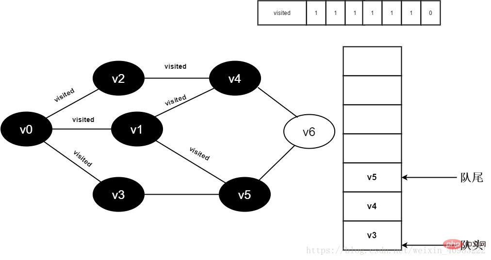
Figure 3-2-12
All adjacent points of 13.v1 have been visited, and the head element of the team v3 dequeues and starts accessing all adjacent points of v3.
Start visiting the v3 neighbor point v0. Because the visited[0] value is 1, no visit will be performed.
Continue to visit v3 neighbor point v5, because the visited[5] value is 1, no visit is performed.
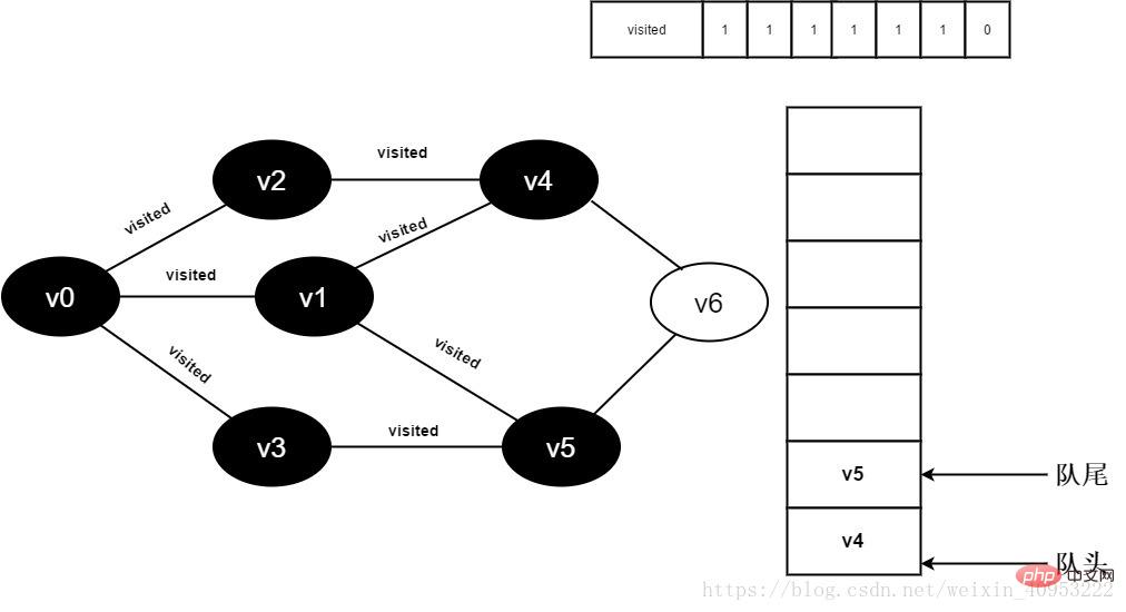
Figure 3-2-13
All adjacent points of 14.v3 have been visited, and The head element v4 is dequeued and begins to visit all adjacent points of v4.
Start visiting the adjacent point v2 of v4. Because the value of visited[2] is 1, no visit will be performed.
Continue to visit the adjacent point v6 of v4, because the value of visited[6] is 0, visit v6, as shown below:
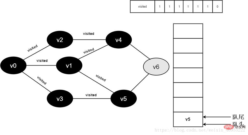
Figure 3-2-14
15. Set the value of visited[6] to 1 and add v6 to the queue.
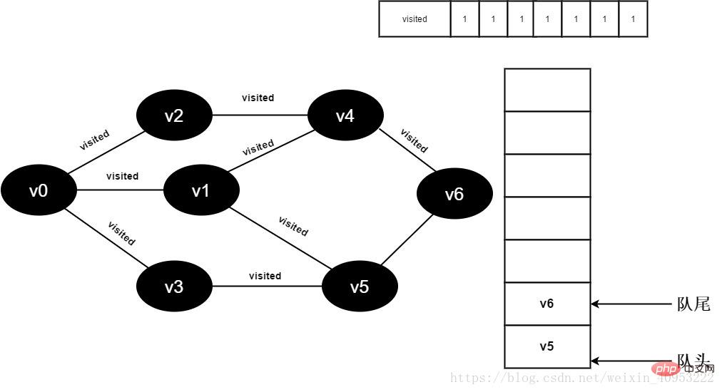
Figure 3-2-15
All adjacent points of 16.v4 have been visited. The head element v5 is dequeued and begins to visit all adjacent points of v5.
Start visiting v5 neighbor point v3. Because the value of visited[3] is 1, no visit will be performed.
Continue to visit v5 neighbor point v6, because the value of visited[6] is 1, no visit is performed.
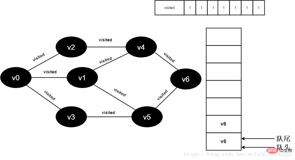
Figure 3-2-16
All adjacent points of 17.v5 have been visited. The head element v6 is dequeued and begins to visit all adjacent points of v6.
Start visiting v6 neighbor point v4. Because the value of visited[4] is 1, no visit will be performed.
Continue to visit the v6 neighbor point v5. Because the value of visited[5] is 1, no visit will be performed.

Figure 3-2-17
18. The queue is empty, exit the loop, and all vertices have been visited.

##Figure 3-2-18
3.3 Details Implementation of the code3.3.1 Use the adjacency matrix to represent the breadth-first search of the graph
/*一些量的定义*/
queue<char> q;				//定义一个队列,使用库函数queue
#define MVNum 100			//表示最大顶点个数
bool visited[MVNum];		        //定义一个visited数组,记录已被访问的顶点
Copy after login
/*邻接矩阵存储表示*/
typedef struct AMGraph
{
	char vexs[MVNum];            //顶点表
	int arcs[MVNum][MVNum];      //邻接矩阵
	int vexnum, arcnum;          //当前的顶点数和边数
}
AMGraph;
Copy after login
/*找到顶点v的对应下标*/
int LocateVex(AMGraph &G, char v)
{
	int i;
	for (i = 0; i < G.vexnum; i++)
		if (G.vexs[i] == v)
			return i;
}
Copy after login/*采用邻接矩阵表示法,创建无向图G*/
int CreateUDG_1(AMGraph &G)
{
int i, j, k;
char v1, v2;
scanf("%d%d", &G.vexnum, &G.arcnum); //输入总顶点数,总边数
getchar(); //获取'\n’,防止其对之后的字符输入造成影响
for (i = 0; i < G.vexnum; i++)
scanf("%c", &G.vexs[i]); //依次输入点的信息
for (i = 0; i < G.vexnum; i++)
for (j = 0; j < G.vexnum; j++)
G.arcs[i][j] = 0; //初始化邻接矩阵边,0表示顶点i和j之间无边
for (k = 0; k < G.arcnum; k++)
{
getchar();
scanf("%c%c", &v1, &v2); //输入一条边依附的顶点
i = LocateVex(G, v1); //找到顶点i的下标
j = LocateVex(G, v2); //找到顶点j的下标
G.arcs[i][j] = G.arcs[j][i] = 1; //1表示顶点i和j之间有边,无向图不区分方向
}
return 1;
}Copy after login/*采用邻接矩阵表示图的广度优先遍历*/
void BFS_AM(AMGraph &G,char v0)
{
/*从v0元素开始访问图*/
int u,i,v,w;
v = LocateVex(G,v0); //找到v0对应的下标
printf("%c ", v0); //打印v0
visited[v] = 1; //顶点v0已被访问
q.push(v0); //将v0入队
while (!q.empty())
{
u = q.front(); //将队头元素u出队,开始访问u的所有邻接点
v = LocateVex(G, u); //得到顶点u的对应下标
q.pop(); //将顶点u出队
for (i = 0; i < G.vexnum; i++)
{
w = G.vexs[i];
if (G.arcs[v][i] && !visited[i])//顶点u和w间有边,且顶点w未被访问
{
printf("%c ", w); //打印顶点w
q.push(w); //将顶点w入队
visited[i] = 1; //顶点w已被访问
}
}
}
}Copy after login
3.3.2 Use the adjacency list to represent the breadth-first search of the graph/*一些量的定义*/ queue<char> q; //定义一个队列,使用库函数queue #define MVNum 100 //表示最大顶点个数 bool visited[MVNum]; //定义一个visited数组,记录已被访问的顶点
/*邻接矩阵存储表示*/
typedef struct AMGraph
{
char vexs[MVNum]; //顶点表
int arcs[MVNum][MVNum]; //邻接矩阵
int vexnum, arcnum; //当前的顶点数和边数
}
AMGraph;/*找到顶点v的对应下标*/
int LocateVex(AMGraph &G, char v)
{
int i;
for (i = 0; i < G.vexnum; i++)
if (G.vexs[i] == v)
return i;
}/*采用邻接矩阵表示法,创建无向图G*/
int CreateUDG_1(AMGraph &G)
{
int i, j, k;
char v1, v2;
scanf("%d%d", &G.vexnum, &G.arcnum); //输入总顶点数,总边数
getchar(); //获取'\n’,防止其对之后的字符输入造成影响
for (i = 0; i < G.vexnum; i++)
scanf("%c", &G.vexs[i]); //依次输入点的信息
for (i = 0; i < G.vexnum; i++)
for (j = 0; j < G.vexnum; j++)
G.arcs[i][j] = 0; //初始化邻接矩阵边,0表示顶点i和j之间无边
for (k = 0; k < G.arcnum; k++)
{
getchar();
scanf("%c%c", &v1, &v2); //输入一条边依附的顶点
i = LocateVex(G, v1); //找到顶点i的下标
j = LocateVex(G, v2); //找到顶点j的下标
G.arcs[i][j] = G.arcs[j][i] = 1; //1表示顶点i和j之间有边,无向图不区分方向
}
return 1;
}/*采用邻接矩阵表示图的广度优先遍历*/
void BFS_AM(AMGraph &G,char v0)
{
/*从v0元素开始访问图*/
int u,i,v,w;
v = LocateVex(G,v0); //找到v0对应的下标
printf("%c ", v0); //打印v0
visited[v] = 1; //顶点v0已被访问
q.push(v0); //将v0入队
while (!q.empty())
{
u = q.front(); //将队头元素u出队,开始访问u的所有邻接点
v = LocateVex(G, u); //得到顶点u的对应下标
q.pop(); //将顶点u出队
for (i = 0; i < G.vexnum; i++)
{
w = G.vexs[i];
if (G.arcs[v][i] && !visited[i])//顶点u和w间有边,且顶点w未被访问
{
printf("%c ", w); //打印顶点w
q.push(w); //将顶点w入队
visited[i] = 1; //顶点w已被访问
}
}
}
}/*找到顶点对应的下标*/
int LocateVex(ALGraph &G, char v)
{
int i;
for (i = 0; i < G.vexnum; i++)
if (v == G.vertices[i].data)
return i;
}Copy after login/*邻接表存储表示*/
typedef struct ArcNode //边结点
{
int adjvex; //该边所指向的顶点的位置
ArcNode *nextarc; //指向下一条边的指针
int info; //和边相关的信息,如权值
}ArcNode;
typedef struct VexNode //表头结点
{
char data;
ArcNode *firstarc; //指向第一条依附该顶点的边的指针
}VexNode,AdjList[MVNum]; //AbjList表示一个表头结点表
typedef struct ALGraph
{
AdjList vertices;
int vexnum, arcnum;
}ALGraph;Copy after login/*采用邻接表表示法,创建无向图G*/
int CreateUDG_2(ALGraph &G)
{
int i, j, k;
char v1, v2;
scanf("%d%d", &G.vexnum, &G.arcnum); //输入总顶点数,总边数
getchar();
for (i = 0; i < G.vexnum; i++) //输入各顶点,构造表头结点表
{
scanf("%c", &G.vertices[i].data); //输入顶点值
G.vertices[i].firstarc = NULL; //初始化每个表头结点的指针域为NULL
}
for (k = 0; k < G.arcnum; k++) //输入各边,构造邻接表
{
getchar();
scanf("%c%c", &v1, &v2); //输入一条边依附的两个顶点
i = LocateVex(G, v1); //找到顶点i的下标
j = LocateVex(G, v2); //找到顶点j的下标
ArcNode *p1 = new ArcNode; //创建一个边结点*p1
p1->adjvex = j; //其邻接点域为j
p1->nextarc = G.vertices[i].firstarc; G.vertices[i].firstarc = p1; // 将新结点*p插入到顶点v1的边表头部
ArcNode *p2 = new ArcNode; //生成另一个对称的新的表结点*p2
p2->adjvex = i;
p2->nextarc = G.vertices[j].firstarc;
G.vertices[j].firstarc = p1;
}
return 1;
}Copy after login
/*采用邻接表表示图的广度优先遍历*/
void BFS_AL(ALGraph &G, char v0)
{
	int u,w,v;
	ArcNode *p;
	printf("%c ", v0);		                                        //打印顶点v0
	v = LocateVex(G, v0);	                                                //找到v0对应的下标
	visited[v] = 1;			                                        //顶点v0已被访问
	q.push(v0);				                                //将顶点v0入队
	while (!q.empty())
	{
		u = q.front();		                                        //将顶点元素u出队,开始访问u的所有邻接点
		v = LocateVex(G, u);                                            //得到顶点u的对应下标
		q.pop();			//将顶点u出队
		for (p = G.vertices[v].firstarc; p; p = p->nextarc)		//遍历顶点u的邻接点
		{
			w = p->adjvex;
			if (!visited[w])	//顶点p未被访问
			{
				printf("%c ", G.vertices[w].data);	        //打印顶点p
				visited[w] = 1;				        //顶点p已被访问
				q.push(G.vertices[w].data);			//将顶点p入队
			}
		}
	}
}
Copy after login
3.4. Non Implementation method of breadth-first traversal of connected graph/*找到顶点对应的下标*/
int LocateVex(ALGraph &G, char v)
{
int i;
for (i = 0; i < G.vexnum; i++)
if (v == G.vertices[i].data)
return i;
}/*邻接表存储表示*/
typedef struct ArcNode //边结点
{
int adjvex; //该边所指向的顶点的位置
ArcNode *nextarc; //指向下一条边的指针
int info; //和边相关的信息,如权值
}ArcNode;
typedef struct VexNode //表头结点
{
char data;
ArcNode *firstarc; //指向第一条依附该顶点的边的指针
}VexNode,AdjList[MVNum]; //AbjList表示一个表头结点表
typedef struct ALGraph
{
AdjList vertices;
int vexnum, arcnum;
}ALGraph;/*采用邻接表表示法,创建无向图G*/
int CreateUDG_2(ALGraph &G)
{
int i, j, k;
char v1, v2;
scanf("%d%d", &G.vexnum, &G.arcnum); //输入总顶点数,总边数
getchar();
for (i = 0; i < G.vexnum; i++) //输入各顶点,构造表头结点表
{
scanf("%c", &G.vertices[i].data); //输入顶点值
G.vertices[i].firstarc = NULL; //初始化每个表头结点的指针域为NULL
}
for (k = 0; k < G.arcnum; k++) //输入各边,构造邻接表
{
getchar();
scanf("%c%c", &v1, &v2); //输入一条边依附的两个顶点
i = LocateVex(G, v1); //找到顶点i的下标
j = LocateVex(G, v2); //找到顶点j的下标
ArcNode *p1 = new ArcNode; //创建一个边结点*p1
p1->adjvex = j; //其邻接点域为j
p1->nextarc = G.vertices[i].firstarc; G.vertices[i].firstarc = p1; // 将新结点*p插入到顶点v1的边表头部
ArcNode *p2 = new ArcNode; //生成另一个对称的新的表结点*p2
p2->adjvex = i;
p2->nextarc = G.vertices[j].firstarc;
G.vertices[j].firstarc = p1;
}
return 1;
}/*采用邻接表表示图的广度优先遍历*/
void BFS_AL(ALGraph &G, char v0)
{
int u,w,v;
ArcNode *p;
printf("%c ", v0); //打印顶点v0
v = LocateVex(G, v0); //找到v0对应的下标
visited[v] = 1; //顶点v0已被访问
q.push(v0); //将顶点v0入队
while (!q.empty())
{
u = q.front(); //将顶点元素u出队,开始访问u的所有邻接点
v = LocateVex(G, u); //得到顶点u的对应下标
q.pop(); //将顶点u出队
for (p = G.vertices[v].firstarc; p; p = p->nextarc) //遍历顶点u的邻接点
{
w = p->adjvex;
if (!visited[w]) //顶点p未被访问
{
printf("%c ", G.vertices[w].data); //打印顶点p
visited[w] = 1; //顶点p已被访问
q.push(G.vertices[w].data); //将顶点p入队
}
}
}
}/*广度优先搜索非连通图*/
void BFSTraverse(AMGraph G)
{
int v;
for (v = 0; v < G.vexnum; v++)
visited[v] = 0; //将visited数组初始化
for (v = 0; v < G.vexnum; v++)
if (!visited[v]) BFS_AM(G, G.vexs[v]); //对尚未访问的顶点调用BFS
}Copy after login
4. Depth-first search4.1 Basic idea of the algorithmDepth-first search is similar to pre-order traversal of a tree, specifically The process is as follows: Preparation: Create a visited array to record all visited vertices. 1. Starting from v0 in the picture, visit v0. 2. Find the first unvisited adjacent point of v0 and visit the vertex. Use this vertex as a new vertex and repeat this step until the vertex just visited has no unvisited adjacent vertices. 3. Return to the previously visited vertex that still has unvisited adjacent points, and continue to visit the next unvisited leading point of the vertex. 4. Repeat steps 2 and 3 until all vertices are visited and the search ends. 4.2 Implementation process of the algorithm1. Initially, all vertices have not been visited, and the visited array is empty. /*广度优先搜索非连通图*/
void BFSTraverse(AMGraph G)
{
int v;
for (v = 0; v < G.vexnum; v++)
visited[v] = 0; //将visited数组初始化
for (v = 0; v < G.vexnum; v++)
if (!visited[v]) BFS_AM(G, G.vexs[v]); //对尚未访问的顶点调用BFS
}
Figure 4-2-1

Figure 4-2-2
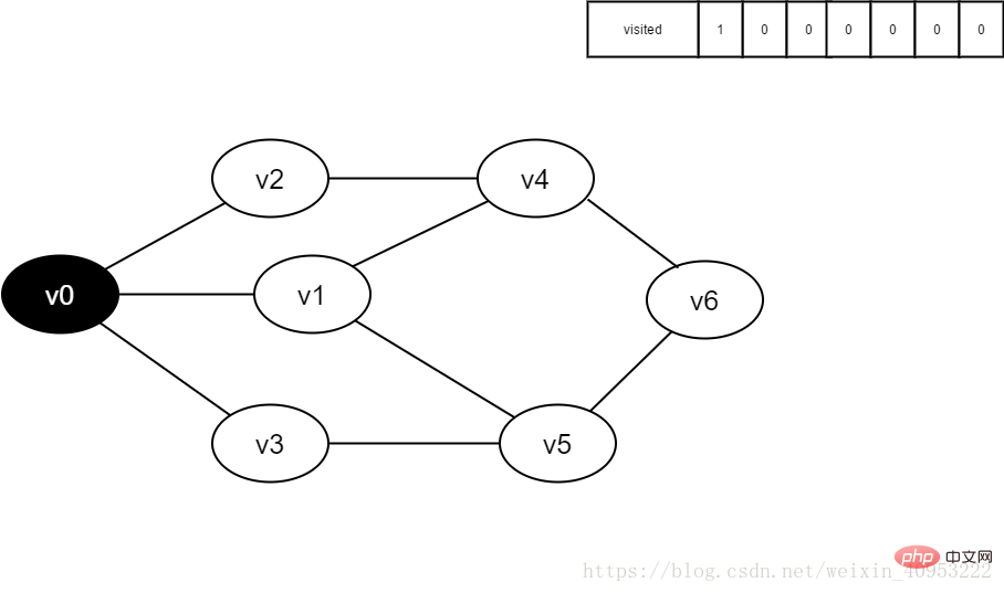
Figure 4-2-3
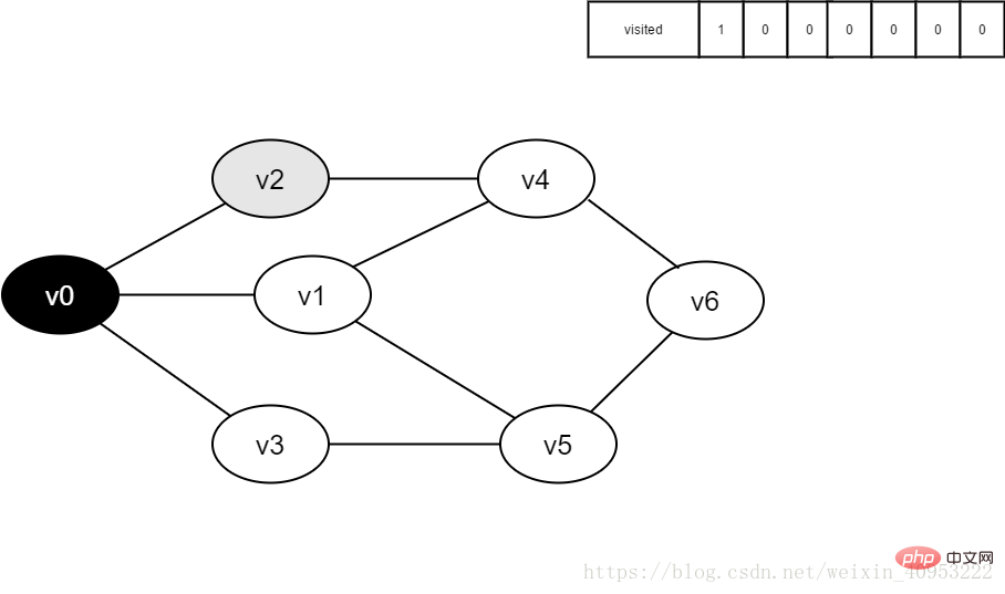
Figure 4-2-4
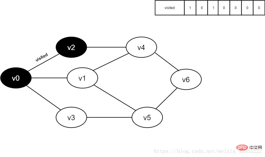
Figure 4-2-5
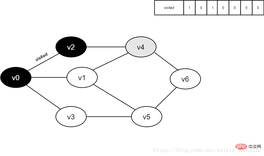
Figure 4-2-6
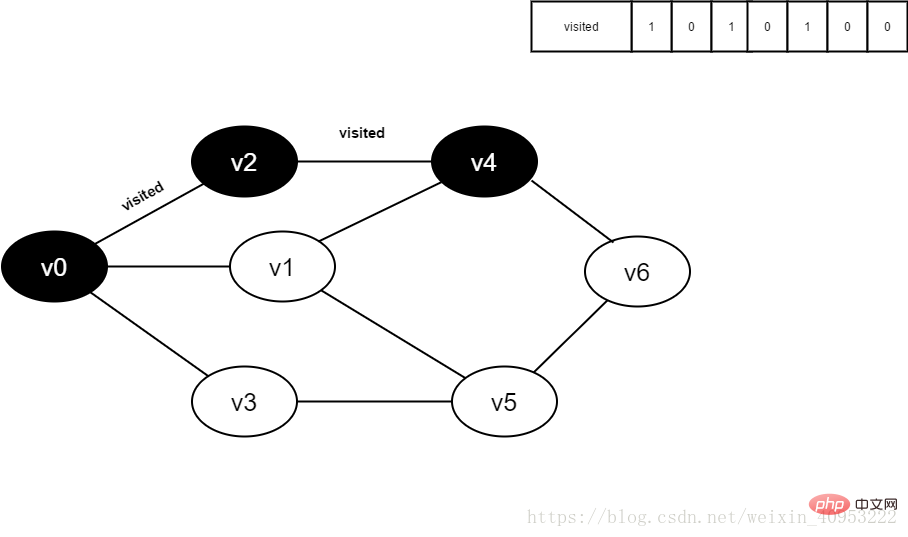
Figure 4-2-7
8. Visit the adjacent point v1 of v4, determine visited[1], and its value is 0, access v1.
Figure 4-2-8
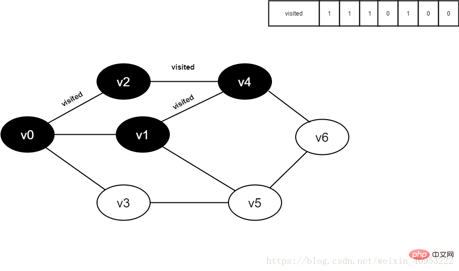
Figure 4-2-9
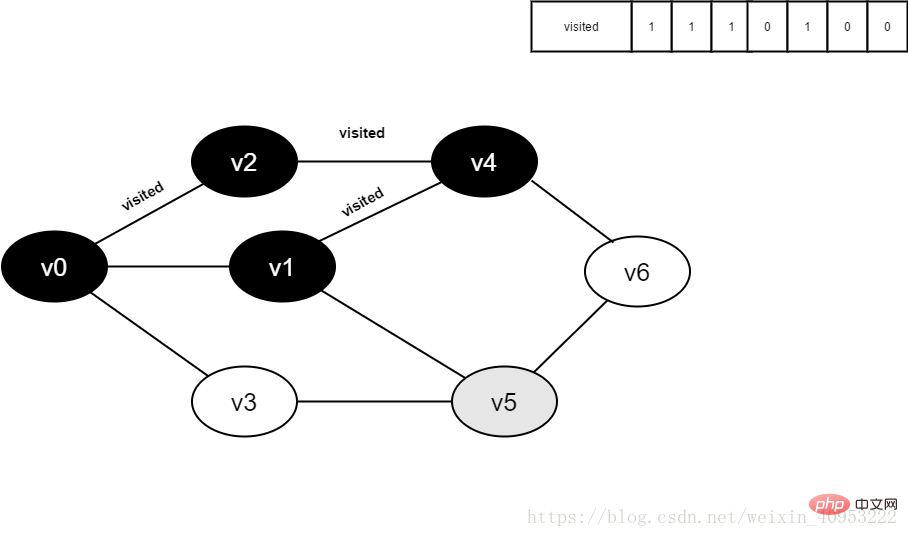
Figure 4-2-10
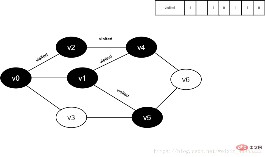
Figure 4-2-11

图4-2-12
13.将visited[1]置为1。
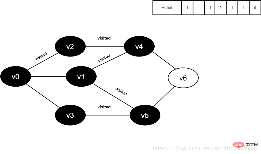
图4-2-13
14.访问v3的邻接点v0,判断visited[0],其值为1,不访问。
继续访问v3的邻接点v5,判断visited[5],其值为1,不访问。
v3所有邻接点均已被访问,回溯到其上一个顶点v5,遍历v5所有邻接点。
访问v5的邻接点v6,判断visited[6],其值为0,访问v6。
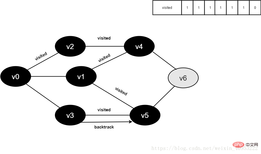
图4-2-14
15.将visited[6]置为1。
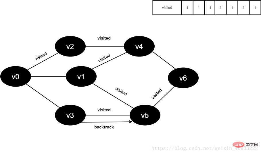
图4-2-15
16.访问v6的邻接点v4,判断visited[4],其值为1,不访问。
访问v6的邻接点v5,判断visited[5],其值为1,不访问。
v6所有邻接点均已被访问,回溯到其上一个顶点v5,遍历v5剩余邻接点。
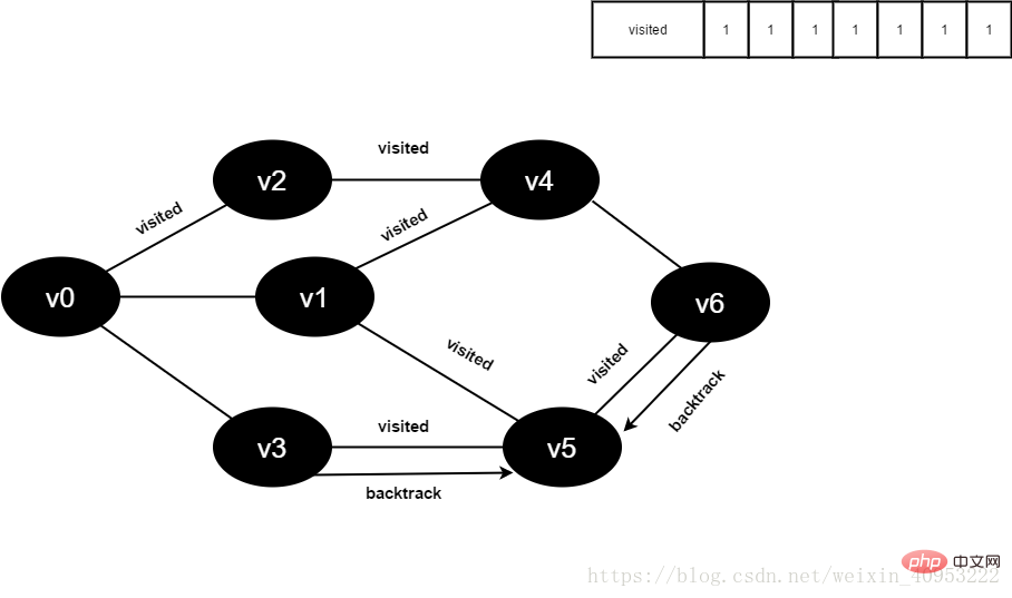
图4-2-16
17.v5所有邻接点均已被访问,回溯到其上一个顶点v1。
v1所有邻接点均已被访问,回溯到其上一个顶点v4,遍历v4剩余邻接点v6。
v4所有邻接点均已被访问,回溯到其上一个顶点v2。
v2所有邻接点均已被访问,回溯到其上一个顶点v1,遍历v1剩余邻接点v3。
v1所有邻接点均已被访问,搜索结束。
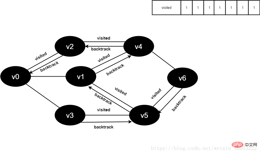
图4-2-17
4.3具体代码实现
4.3.1用邻接矩阵表示图的深度优先搜索
邻接矩阵的创建在上述已描述过,这里不再赘述
void DFS_AM(AMGraph &G, int v)
{
	int w;
	printf("%c ", G.vexs[v]);
	visited[v] = 1;
	for (w = 0; w < G.vexnum; w++)
		if (G.arcs[v][w]&&!visited[w]) //递归调用
			DFS_AM(G,w);
}4.3.2用邻接表表示图的深度优先搜素
邻接表的创建在上述已描述过,这里不再赘述。
void DFS_AL(ALGraph &G, int v)
{
	int w;
	printf("%c ", G.vertices[v].data);
	visited[v] = 1;
	ArcNode *p = new ArcNode;
	p = G.vertices[v].firstarc;
	while (p)
	{
		w = p->adjvex;
		if (!visited[w]) DFS_AL(G, w);
		p = p->nextarc;
	}
}更多相关知识,请访问:PHP中文网!
The above is the detailed content of What is breadth-first traversal of a graph similar to a binary tree?. For more information, please follow other related articles on the PHP Chinese website!

Hot AI Tools

Undresser.AI Undress
AI-powered app for creating realistic nude photos

AI Clothes Remover
Online AI tool for removing clothes from photos.

Undress AI Tool
Undress images for free

Clothoff.io
AI clothes remover

Video Face Swap
Swap faces in any video effortlessly with our completely free AI face swap tool!

Hot Article
Hot Tools

Notepad++7.3.1
Easy-to-use and free code editor

SublimeText3 Chinese version
Chinese version, very easy to use

Zend Studio 13.0.1
Powerful PHP integrated development environment

Dreamweaver CS6
Visual web development tools

SublimeText3 Mac version
God-level code editing software (SublimeText3)
Hot Topics
 1665
1665
 14
1424
52
1322
25
1270
29
1250
24
14
1424
52
1322
25
1270
29
1250
24

 Detailed explanation of binary tree structure in Java
Jun 16, 2023 am 08:58 AM
Detailed explanation of binary tree structure in Java
Jun 16, 2023 am 08:58 AM
Binary trees are a common data structure in computer science and a commonly used data structure in Java programming. This article will introduce the binary tree structure in Java in detail. 1. What is a binary tree? In computer science, a binary tree is a tree structure in which each node has at most two child nodes. Among them, the left child node is smaller than the parent node, and the right child node is larger than the parent node. In Java programming, binary trees are commonly used to represent sorting, searching and improving the efficiency of data query. 2. Binary tree implementation in Java In Java, binary tree
 Print left view of binary tree in C language
Sep 03, 2023 pm 01:25 PM
Print left view of binary tree in C language
Sep 03, 2023 pm 01:25 PM
The task is to print the left node of the given binary tree. First, the user will insert data, thus generating a binary tree, and then print the left view of the resulting tree. Each node can have at most 2 child nodes so this program must iterate over only the left pointer associated with the node if the left pointer is not null it means it will have some data or pointer associated with it otherwise it will be printed and displayed as the left child of the output. ExampleInput:10324Output:102Here, the orange node represents the left view of the binary tree. In the given graph the node with data 1 is the root node so it will be printed and instead of going to the left child it will print 0 and then it will go to 3 and print its left child which is 2 . We can use recursive method to store the level of node
 In C language, print the right view of the binary tree
Sep 16, 2023 pm 11:13 PM
In C language, print the right view of the binary tree
Sep 16, 2023 pm 11:13 PM
The task is to print the right node of the given binary tree. First the user will insert data to create a binary tree and then print a right view of the resulting tree. The image above shows a binary tree created using nodes 10, 42, 93, 14, 35, 96, 57 and 88, with the nodes on the right side of the tree selected and displayed. For example, 10, 93, 57, and 88 are the rightmost nodes of the binary tree. Example Input:1042931435965788Output:10935788 Each node has two pointers, the left pointer and the right pointer. According to this question, the program only needs to traverse the right node. Therefore, the left child of the node does not need to be considered. The right view stores all nodes that are the last node in their hierarchy. Therefore, we can
 How to implement binary tree traversal using Python
Jun 09, 2023 pm 09:12 PM
How to implement binary tree traversal using Python
Jun 09, 2023 pm 09:12 PM
As a commonly used data structure, binary trees are often used to store data, search and sort. Traversing a binary tree is one of the very common operations. As a simple and easy-to-use programming language, Python has many methods to implement binary tree traversal. This article will introduce how to use Python to implement pre-order, in-order and post-order traversal of a binary tree. Basics of Binary Trees Before learning how to traverse a binary tree, we need to understand the basic concepts of a binary tree. A binary tree consists of nodes, each node has a value and two child nodes (left child node and right child node
 The number of isosceles triangles in a binary tree
Sep 05, 2023 am 09:41 AM
The number of isosceles triangles in a binary tree
Sep 05, 2023 am 09:41 AM
A binary tree is a data structure in which each node can have up to two child nodes. These children are called left children and right children respectively. Suppose we are given a parent array representation, you have to use it to create a binary tree. A binary tree may have several isosceles triangles. We have to find the total number of possible isosceles triangles in this binary tree. In this article, we will explore several techniques for solving this problem in C++. Understanding the problem gives you a parent array. You have to represent it in the form of a binary tree so that the array index forms the value of the tree node and the value in the array gives the parent node of that particular index. Note that -1 is always the root parent. Given below is an array and its binary tree representation. Parentarray=[0,-1,3,1,
 Methods and applications of binary tree implementation in PHP
Jun 18, 2023 pm 06:28 PM
Methods and applications of binary tree implementation in PHP
Jun 18, 2023 pm 06:28 PM
In computer science, a binary tree is an important data structure. It consists of nodes and the edges pointing to them, with each node connecting up to two child nodes. Binary trees are widely used in fields such as search algorithms, compilers, databases, and memory management. Many programming languages support the implementation of binary tree data structures, PHP being one of them. This article will introduce how PHP implements binary trees and its applications. Definition of Binary Tree A binary tree is a data structure that consists of nodes and edges pointing to them. Each node is connected to at most two child nodes,
 Detailed explanation of Java binary tree implementation and specific application cases
Jun 15, 2023 pm 11:03 PM
Detailed explanation of Java binary tree implementation and specific application cases
Jun 15, 2023 pm 11:03 PM
Detailed explanation of Java binary tree implementation and specific application cases. Binary tree is a data structure often used in computer science and can perform very efficient search and sort operations. In this article, we will discuss how to implement a binary tree in Java and some of its specific application cases. Definition of Binary Tree Binary tree is a very important data structure, consisting of the root node (the top node of the tree) and several left subtrees and right subtrees. Each node has at most two child nodes, the child node on the left is called the left subtree, and the child node on the right is called the right subtree. If the node does not have
 Binary tree algorithm in PHP and FAQs
Jun 09, 2023 am 09:33 AM
Binary tree algorithm in PHP and FAQs
Jun 09, 2023 am 09:33 AM
With the continuous development of web development, PHP, as a widely used server scripting language, its algorithms and data structures are becoming more and more important. Among these algorithms and data structures, the binary tree algorithm is a very important concept. This article will introduce the binary tree algorithm and its applications in PHP, as well as answers to common questions. What is a binary tree? A binary tree is a tree structure in which each node has at most two child nodes, a left child node and a right child node. If a node has no child nodes, it is called a leaf node. Binary trees are often used for searching