How to create drop down list in Excel: dynamic, editable, searchable

This tutorial shows simple steps to create a drop-down list in Excel: Create from cell ranges, named ranges, Excel tables, other worksheets. You will also learn how to make Excel drop-down menus dynamic, editable, and searchable.

Microsoft Excel is good at organizing and analyzing complex data. One of its most useful features is the ability to create drop-down menus that allow users to select items from predefined lists. The drop-down menu allows for faster, more accurate and more consistent data entry. This article will show you several different ways to create drop-down menus in Excel.

- Excel drop-down list - How to create drop-down list in Excel - From range - From named range - From table - Create dynamic drop-down list - Create dynamic drop-down list in Excel 365 - Add drop-down list from other worksheets - Insert drop-down list from other workbooks - Create searchable drop-down list in Excel 365 - Drop-down list with messages - Editable drop-down list

Excel drop-down list ---------------------- Excel drop-down list , also known as the *drop-down box* or *drop-down menu*, is used to enter data in a spreadsheet from a predefined list of items. When you select a cell that contains the list, a small arrow appears next to the cell, which you can click on to select.

The main purpose of using drop-down lists in Excel is to limit the number of options available to users. In addition, the drop-down list prevents typos and makes data entry faster and more consistent.

How to create a drop-down list in Excel

To create a drop-down list in Excel, use the Data Verification feature. Here are the steps:

1. Select one or more cells that you want the drop-down list to appear. This can be a single cell, a range of cells, or a whole column. To select multiple discontinuous cells, hold down the Ctrl key.
2. On the Data tab, in the Data Tools group, click Data Verification .
3. On the Settings tab of the Data Verification dialog box, do the following:
   • In the Allow box, select List .
   • In the Source box, enter a comma-separated item, either with or without spaces. Or select the range of cells on the worksheet that contains the items.
   • Make sure the drop-down box in the cell is selected (default), otherwise there will be no drop-down arrow next to the cell.
   • Select or clear the Ignore blank option depending on how you want to handle empty cells.
   • When finished, click OK.

Congratulations! You have successfully created a simple drop-down list in Excel. Your users can now click on the arrow next to the cell and select the entry they want.

The drop-down list created with comma-separated values ​​is suitable for small data validation lists that are unlikely to change. For frequently updated lists, it is best to use ranges or tables as sources. Here are detailed step-by-step instructions for each method.

hint. To speed up data entry in Excel tables, you can also use the data entry table.

Create a drop-down menu from cell range

To insert a drop-down list based on the values ​​in the cell range, perform the following steps:

1. First create a list of items that you want to include in the drop-down list. To do this, just enter each item in a separate cell. This can be done in the same worksheet as the drop-down list or in a different worksheet.
2. Select the cell that will contain the list.
3. On the ribbon, click the Data tab > Data Verification .
4. In the Data Verification dialog window , select List from the Allow drop-down menu. Place the cursor in the Source box and select the range of cells that contain the item, or click the collapse dialog icon and select the range. When finished, click OK.

Advantages : You can modify your dropdown list by making changes in the scope of the reference without editing the data validation list itself.

Cons : To add or delete items, you need to update the source scope reference.

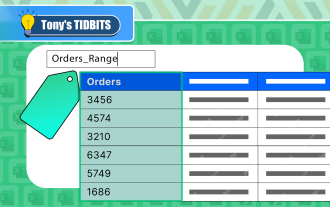
Insert drop-down list from named range

Initially, this method of creating a list of Excel data validation takes a little more time, but it may save more time in the long run.

1. Create a list of items on the worksheet. Values ​​should be entered into a single column or a single row, with no blank cells. hint. It is best to sort items in alphabetical order or in the custom order you want them to appear in the drop-down menu.

2. Create a named range. The fastest way is to select the cell and enter the desired name directly in the Name box . When finished, click Enter to save the newly created named range. For more information, see How to define a name in Excel. For example, let's create a scope called Ingredients :

   

3. Select the cell used to select the list - on the same worksheet as the named range or on a different worksheet.

4. Open the Data Verification Dialog window and configure the rules:

   • In the Allow box, select List .
   • In the Source box, enter an equal sign followed by a range name. In our case, it is =Ingredients .
   • Click OK .

   

Notice. If your named range has at least one blank cell , keep the blank box selected to allow any value to be entered in the validation cell.

Advantages : If you insert multiple drop-down lists in different worksheets, named ranges will make them easier to identify and manage.

Disadvantages : Setting up takes a little more time.

Create a drop-down list from an Excel table

Instead of using named ranges, you can put source data into a fully functional Excel table. Why might you want to use a form? First and foremost, because it allows you to create an extensible dynamic drop-down list that will automatically update when you add or delete items to a table.

To create a dynamic drop-down list from an Excel table, follow these steps:

1. Enter a list item in the table, or use the Ctrl T shortcut key to convert an existing range to a table.
2. Select the cell you want to insert the drop-down list.
3. Open the Data Verification Dialog window.
4. Select a list from the Allow drop-down box.
5. In the Source box, enter a formula that references a specific column in the table, excluding the title cell. To do this, use the INDIRECT function with a structured reference as follows: =INDIRECT("Table_name[Column_name]")
6. When finished, click OK .

For this example, we create a drop-down menu from a column named Ingredients in Table1 :

=INDIRECT("Table1[Ingredients]")

Advantages : Easy and quick way to insert an extensible dynamic drop-down menu in Excel.

Disadvantages : Not found:)

How to create dynamic drop-down list in Excel

If you change items in the selection list frequently, the best way is to create a dynamic drop-down list . In this case, whenever you add or delete an item to the source list, the list will be automatically updated in all included cells.

The fastest way to create a dynamic drop-down list in Excel is to create it from a table, as shown above. This is the default behavior of Excel tables; no additional settings or actions are required.

Another way is to use the regular named range and reference it using the OFFSET formula as described below.

1. In an empty column that does not contain other data, enter the item from the drop-down menu in a separate cell.

2. Create a naming formula. To do this, press Ctrl F3 to open the New Name dialog box. Enter the name you want in the Name box, and then enter the following formula in the Reference to box. =OFFSET(Sheet3!$A$2, 0, 0, COUNTA(Sheet3!$A:$A)-1, 1)

   in:

   • Sheet3 - The name of the worksheet
   • A - The column where the drop-down item is located
   • $A$2 - The cell containing the first item

   

3. After defining the formula name, create a drop-down list based on the naming range in the usual way.

Notice. In this example, cell A1 contains a title and should not be included in the dynamic range. Therefore, we add a -1 correction in the COUNTA function to prevent the addition of blanks at the end of the drop-down list. If there is no other data above the referenced cell, use the COUNTA function without this correction, for example:

=OFFSET(Sheet3!$A$1, 0, 0, COUNTA(Sheet3!$A:$A), 1)

How this formula works

The formula contains two functions - OFFSET and COUNTA. The COUNTA function calculates the number of all non-blank cells in the specified column. OFFSET uses this count as a height parameter, so it returns a reference range that only includes non-empty cells starting from the cell that you provide for the reference parameter that contains the first item.

Notice. To make the formula work correctly, there should be no blank cells between the data entries in the referenced column. If there is other data above the top referenced cell, as shown in the example above, you should subtract the corresponding number of cells from the COUNTA's result.

Advantages : The main advantage of dynamic drop-down lists is that you don't have to change the reference to the named range every time you expand or shrink the source list. You just need to delete or enter a new entry in the source list and your drop-down menu will be automatically updated!

Disadvantages : The setup process is a bit complicated.

Create dynamic drop-down list in Excel 365/2021

Dynamic array Excel has many innovative features that are not available in older versions. One of the new features called UNIQUE can help you create dynamic drop-down lists using simple formulas.

Suppose you have a dataset with many duplicate items, column A in the figure below. Your goal is to add a drop-down list where each item appears only once.

To extract a unique item, use the following formula:

=UNIQUE(A2:A21)

Optionally, you can sort the extracted values ​​alphabetically by wrapping it in the SORT function:

=SORT(UNIQUE(A2:A21))

This dynamic array formula simply enters one cell (E2) and it will automatically expand to the desired number of cells to display all unique items.

Next, you set the drop-down list using the Overflow Range Reference, i.e. the cell address is followed by a hash character. In our example, it is =$E$2# or =Sheet1!$E$2# if the drop-down list is in another worksheet:

The result is an extensible dynamic drop-down list - the UNIQUE function will automatically extract items newly added to the source table, and the overflow range reference will force Excel to update the drop-down list accordingly.

hint. You can use the same method to create a cascading drop-down list in Excel 365. For full details, see Create dynamic dependency drop-down lists in an easy way.

How to create a drop-down list from another worksheet

To insert a drop-down menu that extracts data from different worksheets, you can use the General Scope, Named Scope, or Excel Table:

• When creating a drop-down menu from a named range, make sure that the range of the name is the workbook , and then set up the data verification list in the usual way.
• There is no additional step when creating a dropdown from a table, as the table name/reference is valid throughout the workbook.
• If you insert a drop-down list from a regular scope, include the name of the worksheet in the source reference. In the Data Verification dialog window, place the cursor in the Source box, switch to another worksheet and select the scope that contains the project. Excel will automatically add worksheet names to the reference.

How to create a drop-down list from another workbook

To create a drop-down menu in Excel using a list from another workbook as a source, you will need to define two named ranges - one in the source workbook and the other in the workbook where you want to insert the data validation list. The steps are as follows:

1. In the source workbook, create a named range for the source list, such as Source_list .

2. In the main workbook, define a name that references your source list. For this example, we create a name called Items which references: =SourceFile.xlsx!Source_list

   If the name of the workbook contains spaces or non-alphabetical characters, it must be enclosed in single quotes, as follows:

   ='Source File.xlsx'!Source_list

   For more details, see How to Create External References in Excel.

   

3. In the main workbook, select the cell used to select the list and click the Data tab > Data Verification . In the Source box, refer to the name you created in step 2. In our case, it is =Items.

Notice:

• In order for the drop-down list from another workbook to work, the source workbook must be open.
• The drop-down list created in this way is not automatically updated when items are added or deleted to the source list - you will have to manually modify the source list reference.

How to create a dynamic drop-down list from another workbook

To create a dynamic drop-down list from another workbook, define the formula name in the source workbook using OFFSET formulas, as explained in Create a dynamic drop-down list in Excel. In this case, once any changes are made to the source list, the drop-down menu in another workbook will be updated immediately.

Create a searchable drop-down list in Excel 365

In Excel 365, the data verification list has a great autocomplete feature. To speed up data entry in large lists, just start typing the target word in the drop-down menu cell - the autocomplete algorithm will match the input substring with the items in the drop-down list and show you the matches found. As you enter more characters, the displayed list shrinks, and conversely, when you delete characters, more matches are displayed.

Insert a drop-down list with messages

To display an information message when someone clicks a drop-down list cell, follow the following:

• In the Data Verification dialog box, switch to the Input Messages tab.
• Make sure the display input message option is selected when a cell is selected .
• Enter the title and message in the corresponding field (up to 225 characters).
• Click OK to save the message and close the dialog box.

The resulting drop-down list with message will look something like this:

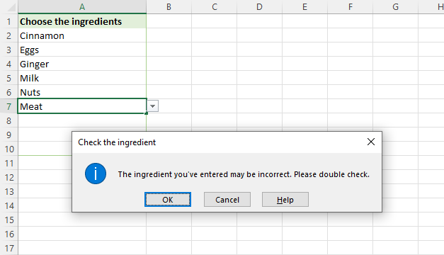
Create an editable drop-down list in Excel

By default, Excel drop-down lists are not editable, i.e. limited to values ​​in the list itself. If you enter any other value, an error alert will be displayed. However, you can allow the user to enter their own values. The method is as follows:

1. Open the Data Verification Dialog window.
2. On the Error Alerts tab, uncheck the Show Error Alerts box after entering invalid data .

Technically, this turns the drop-down list into a combo box . The term "combo box" refers to an editable drop-down list that allows the user to select a value from a predefined list or enter a custom value directly into the box.

Optionally, you can display a warning message when someone tries to enter a value that is not in the list:

1. On the Error Alerts tab, select the Show Error Alerts option after entering invalid data .
2. Select a message or warning from the Style box and enter the title and message text.
   • Information messages are best used when there is no problem with the user entering custom values.
   • A warning message will induce the user to select an item from the drop-down box instead of entering his own data, although it does not prohibit this.

Here is what the editable Excel drop-down list with warning messages actually does:

hint. If you are not sure what title or message text to enter, you can leave the field blank. In this case, Excel will display the default alert " This value does not meet the data validation limit defined for this cell ".

This is how to create a simple dropdown list in Excel. In the next article, we will explore this topic further and learn how to insert a cascading (dependency) drop-down list with conditional data validation. Please continue to pay attention, thanks for reading!

Exercise workbook download

Excel drop-down list - Example (.xlsx file)

The above is the detailed content of How to create drop down list in Excel: dynamic, editable, searchable. For more information, please follow other related articles on the PHP Chinese website!