

How to highlight top 3, 5, 10 values in Excel

This tutorial demonstrates how to highlight top or bottom N values in an Excel dataset using conditional formatting. We'll explore Excel's built-in tools and create custom rules using formulas for greater flexibility.
Methods for Highlighting Top/Bottom Values:
We'll cover three approaches: using built-in rules, enhancing formatting options, and employing formulas for dynamic control.
1. Built-in Top/Bottom Rules:
This is the quickest method for highlighting a fixed number (e.g., top 3, bottom 10) of values.
- Select your data range.
- Go to the Home tab, click Conditional Formatting, then Top/Bottom Rules, and choose either Top 10 Items or Bottom 10 Items.
- Specify the number of items to highlight and select a formatting style. You can customize the formatting using Custom Format.

2. Enhanced Formatting Options:
For more control over the appearance, create a new rule:
- Select your data range.
- Go to Conditional Formatting > New Rule.
- Choose "Format only top or bottom ranked values".
- Select Top or Bottom, enter the number of values, and click Format to customize the font, border, and fill.

3. Formula-Based Conditional Formatting:
This provides the most flexibility, allowing you to change the number of highlighted values without modifying the rule itself.
- Create input cells (e.g., F2 for top N, F3 for bottom N). Enter the desired number of values.
- Select your data range (e.g., A2:C8).
- Go to Conditional Formatting > New Rule > "Use a formula to determine which cells to format".
- Use the following formulas:
-
Top N:
=A2>=LARGE($A$2:$C$8,$F$2) -
Bottom N:
=A2
-
Top N:
- Click Format to choose your formatting style.

These formulas use LARGE and SMALL functions to dynamically determine the threshold values. Absolute references ($) lock the range and input cells, while the relative reference (A2) allows the formula to apply correctly to each cell in the range.
Highlighting Rows Based on Column Values:
To highlight entire rows based on top/bottom N values in a specific column (e.g., column B):
-
Top N Rows:
=$B2>=LARGE($B$2:$B$15,$E$2) -
Bottom N Rows:
=$B2
Apply these formulas to the entire table (excluding the header row).

Highlighting Top N Values in Each Row:
For highlighting the top N values within each row across multiple columns, use this formula:
=B2>=LARGE($B2:$G2,3)
Apply this to the entire numeric data range (e.g., B2:G10).

This formula uses relative row references and absolute column references to correctly compare values within each row.
Downloadable Practice Workbook: Highlight top or bottom values in Excel (.xlsx file)
The above is the detailed content of How to highlight top 3, 5, 10 values in Excel. For more information, please follow other related articles on the PHP Chinese website!

Hot AI Tools

Undresser.AI Undress
AI-powered app for creating realistic nude photos

AI Clothes Remover
Online AI tool for removing clothes from photos.

Undress AI Tool
Undress images for free

Clothoff.io
AI clothes remover

Video Face Swap
Swap faces in any video effortlessly with our completely free AI face swap tool!

Hot Article
Hot Tools

Notepad++7.3.1
Easy-to-use and free code editor

SublimeText3 Chinese version
Chinese version, very easy to use

Zend Studio 13.0.1
Powerful PHP integrated development environment

Dreamweaver CS6
Visual web development tools

SublimeText3 Mac version
God-level code editing software (SublimeText3)
Hot Topics


 How to add calendar to Outlook: shared, Internet calendar, iCal file
Apr 03, 2025 am 09:06 AM
How to add calendar to Outlook: shared, Internet calendar, iCal file
Apr 03, 2025 am 09:06 AM
This article explains how to access and utilize shared calendars within the Outlook desktop application, including importing iCalendar files. Previously, we covered sharing your Outlook calendar. Now, let's explore how to view calendars shared with
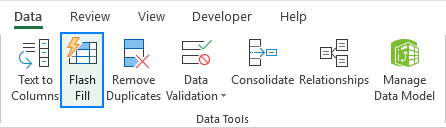 How to use Flash Fill in Excel with examples
Apr 05, 2025 am 09:15 AM
How to use Flash Fill in Excel with examples
Apr 05, 2025 am 09:15 AM
This tutorial provides a comprehensive guide to Excel's Flash Fill feature, a powerful tool for automating data entry tasks. It covers various aspects, from its definition and location to advanced usage and troubleshooting. Understanding Excel's Fla
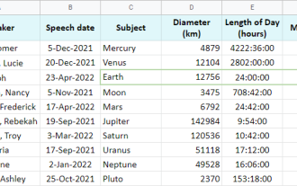
 MEDIAN formula in Excel - practical examples
Apr 11, 2025 pm 12:08 PM
MEDIAN formula in Excel - practical examples
Apr 11, 2025 pm 12:08 PM
This tutorial explains how to calculate the median of numerical data in Excel using the MEDIAN function. The median, a key measure of central tendency, identifies the middle value in a dataset, offering a more robust representation of central tenden
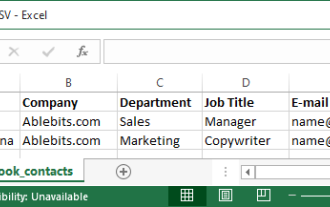 How to import contacts to Outlook (from CSV and PST file)
Apr 02, 2025 am 09:09 AM
How to import contacts to Outlook (from CSV and PST file)
Apr 02, 2025 am 09:09 AM
This tutorial demonstrates two methods for importing contacts into Outlook: using CSV and PST files, and also covers transferring contacts to Outlook Online. Whether you're consolidating data from an external source, migrating from another email pro
 How to use Google Sheets QUERY function – standard clauses and an alternative tool
Apr 02, 2025 am 09:21 AM
How to use Google Sheets QUERY function – standard clauses and an alternative tool
Apr 02, 2025 am 09:21 AM
This comprehensive guide unlocks the power of Google Sheets' QUERY function, often hailed as the most potent spreadsheet function. We'll dissect its syntax and explore its various clauses to master data manipulation. Understanding the Google Sheet
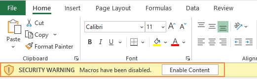 How to enable and disable macros in Excel
Apr 02, 2025 am 09:05 AM
How to enable and disable macros in Excel
Apr 02, 2025 am 09:05 AM
This article explores how to enable macros in Excel, covering macro security basics and safe VBA code execution. Macros, like any technology, have dual potential—beneficial automation or malicious use. Excel's default setting disables macros for sa
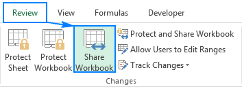 Excel shared workbook: How to share Excel file for multiple users
Apr 11, 2025 am 11:58 AM
Excel shared workbook: How to share Excel file for multiple users
Apr 11, 2025 am 11:58 AM
This tutorial provides a comprehensive guide to sharing Excel workbooks, covering various methods, access control, and conflict resolution. Modern Excel versions (2010, 2013, 2016, and later) simplify collaborative editing, eliminating the need to m
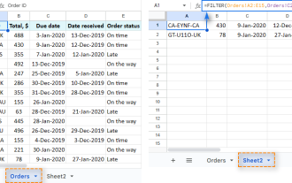 How to use Google Sheets FILTER function
Apr 02, 2025 am 09:19 AM
How to use Google Sheets FILTER function
Apr 02, 2025 am 09:19 AM
Unlock the Power of Google Sheets' FILTER Function: A Comprehensive Guide Tired of basic Google Sheets filtering? This guide unveils the capabilities of the FILTER function, offering a powerful alternative to the standard filtering tool. We'll explo
