

Excel에서 테이블을 만드는 방법

How to Make a Table in Excel
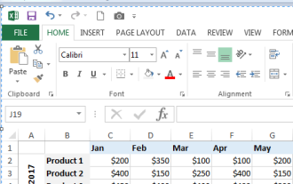
Creating a table in Excel is a straightforward process that can help you organize and analyze your data more effectively. Here are the steps to create a basic table:
- Open Excel: Start by opening Microsoft Excel on your computer.
- Enter Data: Input your data into the worksheet. Ensure that your data is organized in rows and columns, with headers at the top of each column.
- Select Data: Click and drag to select the range of cells that you want to convert into a table. Make sure to include the headers.
-
Insert Table: Go to the "Insert" tab on the ribbon, and click on the "Table" button. Alternatively, you can use the shortcut
Ctrl + T. - Confirm Table Range: A dialog box will appear, asking you to confirm the range of cells you've selected. Ensure the "My table has headers" checkbox is ticked if your data includes headers, then click "OK."
- Table Creation: Excel will automatically format your selected data into a table, with filter arrows in the header row for easy data sorting and filtering.
What are the Steps to Format a Table in Excel?
Formatting a table in Excel helps improve readability and can make your data more visually appealing. Here are the steps to format a table:
- Select the Table: Click anywhere inside the table you want to format.
- Access Table Tools: Once the table is selected, the "Table Design" tab will appear on the ribbon. Click on it to access various formatting options.
- Choose a Table Style: Under the "Table Styles" section, you'll see various pre-designed table styles. Click on one to apply it to your table. You can hover over the styles to see a live preview before making a selection.
- Customize Table Style: If you want more control over the formatting, click on the "More" button (it looks like a small arrow) in the "Table Styles" section to expand the gallery. You can also use the "New Table Style" option to create a custom style.
- Adjust Table Elements: Use the options in the "Table Style Options" group to toggle features like header row, total row, banded rows, and banded columns on or off.
- Resize the Table: If you need to adjust the size of your table, you can drag the resize handle in the bottom-right corner of the table, or use the "Resize Table" option found under the "Table Design" tab.
- Format Cells: To further customize individual cells, rows, or columns, you can use the standard Excel formatting tools found in the "Home" tab, such as font size, cell color, and borders.
How Can I Customize the Style of a Table in Excel?
Customizing the style of a table in Excel allows you to tailor its appearance to suit your preferences or to meet specific requirements. Here's how you can do it:
- Select the Table: Click inside the table to select it.
- Open Table Design: Go to the "Table Design" tab on the ribbon.
- Select a Predefined Style: Browse through the "Table Styles" gallery and select a style that suits your needs. Hover over the styles to see a live preview.
- Create a Custom Style: If none of the predefined styles meet your requirements, click on "New Table Style" in the "Table Styles" gallery. This opens a dialog box where you can define every aspect of the table's appearance, including font, colors, and border styles.
- Modify Table Elements: Use the "Table Style Options" to toggle on or off elements such as header row, total row, first column, last column, banded rows, and banded columns.
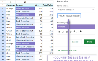
- Adjust Cell Formatting: Use the formatting tools in the "Home" tab to change the font, size, color, and alignment of cells within the table. You can also apply conditional formatting to highlight specific data based on certain criteria.
- Save Custom Style: If you've created a custom style that you want to use in the future, click "New Table Style," name your style, and click "OK." Your custom style will then be available in the "Table Styles" gallery.
What Functions Can I Use to Analyze Data Within an Excel Table?
Excel offers a variety of functions and tools that can be used to analyze data within a table. Here are some useful functions and their applications:
-
SUM: This function calculates the total of selected numerical values. For example,
=SUM(Table1[Column1])will sum all values in Column1 of Table1. -
AVERAGE: This function calculates the average of selected numerical values. For instance,
=AVERAGE(Table1[Column1])will find the average of all values in Column1 of Table1. -
MIN and MAX: These functions find the minimum and maximum values in a range. For example,
=MIN(Table1[Column1])and=MAX(Table1[Column1])will return the lowest and highest values in Column1, respectively. -
COUNT and COUNTA: These functions count the number of cells that contain numbers or any type of data, respectively. For instance,
=COUNT(Table1[Column1])will count the number of cells with numerical values in Column1, while=COUNTA(Table1[Column1])will count all non-empty cells. -
VLOOKUP and HLOOKUP: These functions allow you to search for a value in a table and return a corresponding value from another column or row. For example,
=VLOOKUP(value, Table1, column_index, FALSE)will look up a value in Table1 and return data from the specified column. -
INDEX and MATCH: These functions can be used together to perform more flexible lookups than VLOOKUP or HLOOKUP.
=INDEX(Table1[Column1], MATCH(value, Table1[Column2], 0))will find a value in Column2 and return the corresponding value from Column1. -
SUBTOTAL: This function calculates a subtotal in a list or database, ignoring rows hidden by filters. For instance,
=SUBTOTAL(9, Table1[Column1])will sum all visible values in Column1. - PivotTable: While not a function, PivotTables are powerful tools for summarizing, analyzing, exploring, and presenting data. You can create a PivotTable from your Excel table by selecting the table, going to the "Insert" tab, and clicking on "PivotTable."
Using these functions and tools, you can perform comprehensive data analysis within an Excel table, helping you to make more informed decisions based on your data.
위 내용은 Excel에서 테이블을 만드는 방법의 상세 내용입니다. 자세한 내용은 PHP 중국어 웹사이트의 기타 관련 기사를 참조하세요!

핫 AI 도구

Undresser.AI Undress
사실적인 누드 사진을 만들기 위한 AI 기반 앱

AI Clothes Remover
사진에서 옷을 제거하는 온라인 AI 도구입니다.

Undress AI Tool
무료로 이미지를 벗다

Clothoff.io
AI 옷 제거제

Video Face Swap
완전히 무료인 AI 얼굴 교환 도구를 사용하여 모든 비디오의 얼굴을 쉽게 바꾸세요!

인기 기사
뜨거운 도구

메모장++7.3.1
사용하기 쉬운 무료 코드 편집기

SublimeText3 중국어 버전
중국어 버전, 사용하기 매우 쉽습니다.

스튜디오 13.0.1 보내기
강력한 PHP 통합 개발 환경

드림위버 CS6
시각적 웹 개발 도구

SublimeText3 Mac 버전
신 수준의 코드 편집 소프트웨어(SublimeText3)


 플래시 채우기를 사용하는 방법 예제와 함께 Excel
Apr 05, 2025 am 09:15 AM
플래시 채우기를 사용하는 방법 예제와 함께 Excel
Apr 05, 2025 am 09:15 AM
이 튜토리얼은 데이터 입력 작업을 자동화하기위한 강력한 도구 인 Excel의 Flash Clone 기능에 대한 포괄적 인 안내서를 제공합니다. 정의 및 위치에서 고급 사용 및 문제 해결에 이르기까지 다양한 측면을 다룹니다. Excel의 FLA 이해
 Excel의 중간 공식 - 실제 예
Apr 11, 2025 pm 12:08 PM
Excel의 중간 공식 - 실제 예
Apr 11, 2025 pm 12:08 PM
이 튜토리얼은 중간 기능을 사용하여 Excel에서 수치 데이터의 중앙값을 계산하는 방법을 설명합니다. 중앙 경향의 주요 척도 인 중앙값은 데이터 세트의 중간 값을 식별하여 Central Tenden의보다 강력한 표현을 제공합니다.
 Excel을 철자하는 방법
Apr 06, 2025 am 09:10 AM
Excel을 철자하는 방법
Apr 06, 2025 am 09:10 AM
이 튜토리얼은 Excel의 맞춤법 검사를위한 다양한 방법과 같은 수동 점검, VBA 매크로 및 특수 도구를 사용합니다. 셀, 범위, 워크 시트 및 전체 통합 문서의 철자 확인을 배우십시오. Excel은 워드 프로세서는 아니지만 Spel
 Excel 공유 통합 문서 : 여러 사용자를위한 Excel 파일을 공유하는 방법
Apr 11, 2025 am 11:58 AM
Excel 공유 통합 문서 : 여러 사용자를위한 Excel 파일을 공유하는 방법
Apr 11, 2025 am 11:58 AM
이 튜토리얼은 다양한 방법, 액세스 제어 및 갈등 해결을 다루는 Excel 통합 문서 공유에 대한 포괄적 인 안내서를 제공합니다. Modern Excel 버전 (2010, 2013, 2016 및 이후) 협업 편집을 단순화하여 M에 대한 필요성을 제거합니다.
 Excel : 그룹 행 자동 또는 수동으로 행을 붕괴하고 확장합니다.
Apr 08, 2025 am 11:17 AM
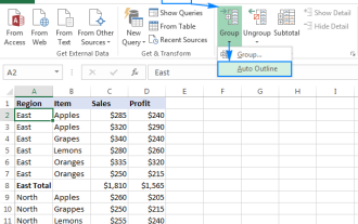
Excel : 그룹 행 자동 또는 수동으로 행을 붕괴하고 확장합니다.
Apr 08, 2025 am 11:17 AM
이 튜토리얼은 행을 그룹화하여 복잡한 Excel 스프레드 시트를 간소화하여 데이터를보다 쉽게 분석 할 수 있도록하는 방법을 보여줍니다. 행 그룹을 신속하게 숨기거나 보여주고 전체 개요를 특정 수준으로 붕괴시키는 법을 배우십시오. 크고 상세한 스프레드 시트가 될 수 있습니다
 Excel의 절대 값 : 공식 예제와 함께 ABS 기능
Apr 06, 2025 am 09:12 AM
Excel의 절대 값 : 공식 예제와 함께 ABS 기능
Apr 06, 2025 am 09:12 AM
이 튜토리얼은 절대 값의 개념을 설명하고 데이터 세트 내에서 절대 값을 계산하기위한 ABS 기능의 실질적인 Excel 응용 프로그램을 보여줍니다. 숫자는 긍정적이거나 부정적 일 수 있지만 때로는 양수 값 만 필요합니다.
 Excel을 JPG로 변환하는 방법 - 이미지 파일로 .xls 또는 .xlsx를 저장
Apr 11, 2025 am 11:31 AM
Excel을 JPG로 변환하는 방법 - 이미지 파일로 .xls 또는 .xlsx를 저장
Apr 11, 2025 am 11:31 AM
이 자습서는 .xls 파일을 .jpg 이미지로 변환하는 다양한 방법을 탐색하여 내장 된 Windows 도구와 무료 온라인 변환기를 모두 포함합니다. 프레젠테이션을 만들거나 스프레드 시트 데이터를 단단히 공유하거나 문서를 디자인해야합니까? YO를 변환합니다
 Google 스프레드 시트 Countif 기능은 공식 예제와 함께합니다
Apr 11, 2025 pm 12:03 PM
Google 스프레드 시트 Countif 기능은 공식 예제와 함께합니다
Apr 11, 2025 pm 12:03 PM
마스터 Google Sheets Countif : 포괄적 인 가이드 이 안내서는 Google 시트의 다목적 카운티프 기능을 탐색하여 간단한 셀 카운팅 이외의 응용 프로그램을 보여줍니다. 우리는 정확하고 부분적인 경기에서 Han에 이르기까지 다양한 시나리오를 다룰 것입니다.
