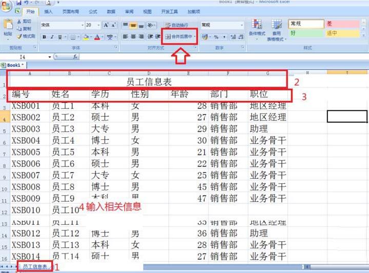
1、打开excel空白表,把sheet1命名为员工信息表——合并a1:g1并居中,输入:员工信息表——a2:g2分别输入编号、姓名、学历、性别、年龄、部门、职位——然后输入各列的相关内容。
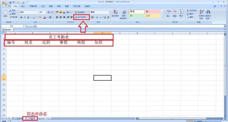
2、制作员工考勤表。双击sheet2重命名为员工考勤表——选择A1:F1——选择合并并居中,输入员工考勤表——在A2:F2分别输入编号、姓名、迟到、事假、病假、加班。
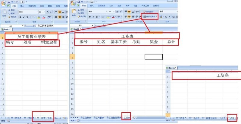
3、按照上述操作继续制员工销售业绩表(主要列的内容为编号、姓名、销量金额)——工资表主要列的内容为编号、姓名、基本工资、考勤、奖金、总计——工资条表(主要合并A1:F1,输入工资条,其它不用输入)。
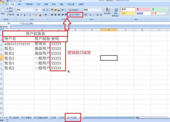
4、制作用记权限表,分配管理编辑表格的权限人员,新建一个表格命名为用户权限表——选择A1:A3合并居中——输入用户权限——A2:A3分别输入用户名、用户级别和密码。
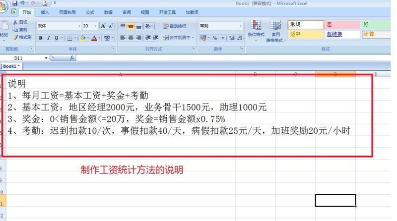
5、制作一张工资说明表,说明具体工作计算,发每月工资中基本工资的计算办法、奖金和考勤的奖罚处理办法等。
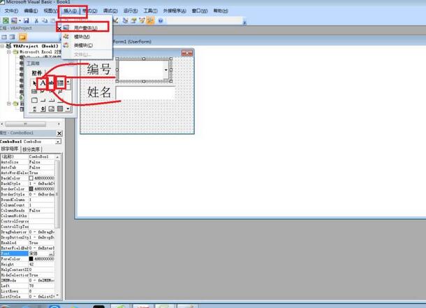
6、这样表格制作完成,同时按ALT+F11打开,点击插入——窗体,去设计记录窗体并录入到相关表中。
以上就是Excel制作人事工资管理系统的操作方法的详细内容,更多请关注php中文网其它相关文章!

全网最新最细最实用WPS零基础入门到精通全套教程!带你真正掌握WPS办公! 内含Excel基础操作、函数设计、数据透视表等

 广告
广告
![ThinkPHP5快速开发企业站点[全程实录]](https://img.php.cn/upload/course/000/000/068/6253d918a3ce7278.png)

Copyright 2014-2025 https://www.php.cn/ All Rights Reserved | php.cn | 湘ICP备2023035733号


 670
670