
 Software Tutorial
Office Software
How to find the same records in two EXCEL tables and count them
Software Tutorial
Office Software
How to find the same records in two EXCEL tables and count them
How to find the same records in two EXCEL tables and count them

I have two EXCEL tables. How do I count the same records in these two tables?
Step 1: Copy all phone numbers in Table 1 and Table 2 to column A of Table 3. The first line of Table 3 is the header, and the second line starts with all the phone numbers, a total of 50,000 lines.
Step 2: Enter the number 1 in column B of Table 3, and use the formula "=COUNTA(A:A)" to fill the cells in column A to count the number of names in column A.
Step 3: Enter the formula SUMIF($B$2:$B$50000,A1,$B$2:$B$50000) in cell C2 of the table. Through this formula, you can get the number of duplicate names in the cells in column A. frequency. When the result is 1, it means there is no repetition. When it is greater than 1, it means there is repetition and the number of repetitions is displayed.
Step 4: Perform automatic filtering in column C of Table 3. The filtering should be based on the current data. For example, filtering "2" means selecting phone numbers repeated twice, and then filtering a phone number from column A. Number (because there may be many duplicate phone numbers, it is best to process them one by one to avoid errors). After deleting the remaining ones, the formula will automatically get "1". After all column A is displayed, it will show that there is no processing. Phone numbers that are repeated twice can be processed in the same way.
When all the data in column C is "1", the remaining phone numbers in column A are the only phone numbers without duplication.
Maybe a little troublesome, but still very accurate.
Also, I borrowed other people’s methods and showed them to you:
Step 1: First copy all the phone numbers in Table 1 and Table 2 to column B of Table 3, set row number 1 as the header, row number 2 to row number 50000 as all phone numbers;
Step 2: Enter the formula =IF(COUNTIF(B$2:B2,B2)=1,B2,"")
in A2Then drag B2 towards fill to A50000
What is displayed are the phone numbers that are not repeated, and the repeated phone numbers are blank cells.
Copy A2:A50000, then right-click - Paste Special - Value, sort ascending and descending, and then clear the contents of column B.
How to find the corresponding information of duplicate cells in two EXCEL tables
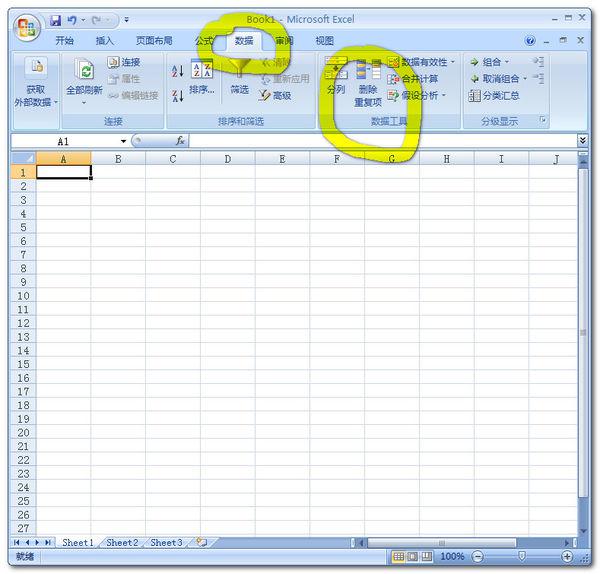
If you want to use the 2003 version, just use the perspective mentioned above. If it is the 2007 version, there is an item in the data tab to delete duplicates. The specific operation is as follows:
1. Select the table you want to operate
2. Open the data tab
3.
4. Then select the Remove Duplicates option
5.
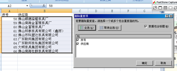
6. Just select the column you want to remove duplicates from. If it's in column B, select the title you wrote in column B. I wrote as supplier here. So select the hook before the supplier and remove the hook before the serial number. Just click OK.
7. The last and most important point is that your repeated names must be exactly the same. As you said, it is the same supplier, but the names are not exactly the same, such as Jinfuya Furniture and Federal. The names of the suppliers are not exactly the same, so you just have to search and replace them with the same name. Finally I hope it helps you.
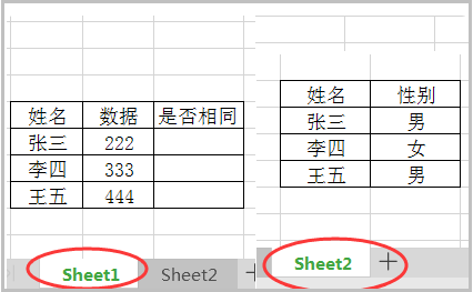
How to compare two excel tables with some identical data in the two tables
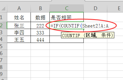
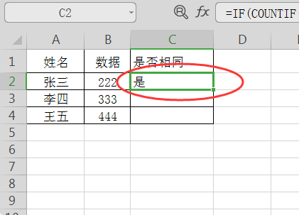
1. Open the excel table, put data one on "Sheet1" and data two on "Sheet2".
2. Enter in cell C2 of sheet1: =IF(COUNTIF(.
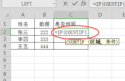
3. Switch to the column in Sheet2 that needs to be queried, and then select the entire column.
4. At this time, the formula in cell C2 in the Sheet1 table automatically changes to: =IF(COUNTIF(Sheet2!A:A.
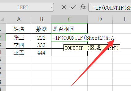
5. Keep the operation interface in Sheet1 and enter the comma under the English characters after the formula: =if(COUNTIF(Sheet2!A:A, .
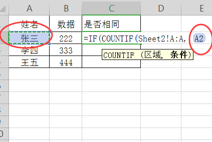
6. In sheet1, select cell A2 with the mouse, and the formula becomes: =IF(COUNTIF(Sheet2!A:A,Sheet1!A2.
7. Next, manually complete the formula in English: =IF(COUNTIF(Sheet2!A:A,Sheet1!A2)>0, "Yes", "No").
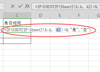
8. Click Enter to get the formula judgment result.
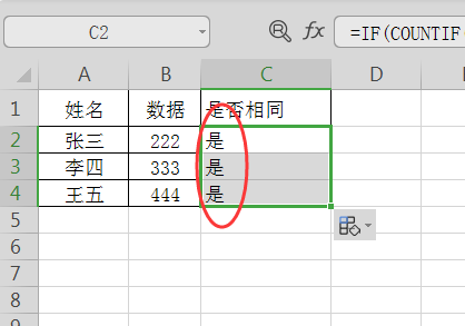
9. Simply pull down the cell with the mouse to complete all judgments.
The above is the detailed content of How to find the same records in two EXCEL tables and count them. For more information, please follow other related articles on the PHP Chinese website!

Hot AI Tools

Undresser.AI Undress
AI-powered app for creating realistic nude photos

AI Clothes Remover
Online AI tool for removing clothes from photos.

Undress AI Tool
Undress images for free

Clothoff.io
AI clothes remover

Video Face Swap
Swap faces in any video effortlessly with our completely free AI face swap tool!

Hot Article
Hot Tools

Notepad++7.3.1
Easy-to-use and free code editor

SublimeText3 Chinese version
Chinese version, very easy to use

Zend Studio 13.0.1
Powerful PHP integrated development environment

Dreamweaver CS6
Visual web development tools

SublimeText3 Mac version
God-level code editing software (SublimeText3)
Hot Topics
 1670
1670
 14
1428
52
1329
25
1274
29
1256
24
14
1428
52
1329
25
1274
29
1256
24

 If You Don't Rename Tables in Excel, Today's the Day to Start
Apr 15, 2025 am 12:58 AM
If You Don't Rename Tables in Excel, Today's the Day to Start
Apr 15, 2025 am 12:58 AM
Quick link Why should tables be named in Excel How to name a table in Excel Excel table naming rules and techniques By default, tables in Excel are named Table1, Table2, Table3, and so on. However, you don't have to stick to these tags. In fact, it would be better if you don't! In this quick guide, I will explain why you should always rename tables in Excel and show you how to do this. Why should tables be named in Excel While it may take some time to develop the habit of naming tables in Excel (if you don't usually do this), the following reasons illustrate today
 How to change Excel table styles and remove table formatting
Apr 19, 2025 am 11:45 AM
How to change Excel table styles and remove table formatting
Apr 19, 2025 am 11:45 AM
This tutorial shows you how to quickly apply, modify, and remove Excel table styles while preserving all table functionalities. Want to make your Excel tables look exactly how you want? Read on! After creating an Excel table, the first step is usual
 Excel MATCH function with formula examples
Apr 15, 2025 am 11:21 AM
Excel MATCH function with formula examples
Apr 15, 2025 am 11:21 AM
This tutorial explains how to use MATCH function in Excel with formula examples. It also shows how to improve your lookup formulas by a making dynamic formula with VLOOKUP and MATCH. In Microsoft Excel, there are many different lookup/ref
 Excel: Compare strings in two cells for matches (case-insensitive or exact)
Apr 16, 2025 am 11:26 AM
Excel: Compare strings in two cells for matches (case-insensitive or exact)
Apr 16, 2025 am 11:26 AM
The tutorial shows how to compare text strings in Excel for case-insensitive and exact match. You will learn a number of formulas to compare two cells by their values, string length, or the number of occurrences of a specific character, a
 How to Make Your Excel Spreadsheet Accessible to All
Apr 18, 2025 am 01:06 AM
How to Make Your Excel Spreadsheet Accessible to All
Apr 18, 2025 am 01:06 AM
Improve the accessibility of Excel tables: A practical guide When creating a Microsoft Excel workbook, be sure to take the necessary steps to make sure everyone has access to it, especially if you plan to share the workbook with others. This guide will share some practical tips to help you achieve this. Use a descriptive worksheet name One way to improve accessibility of Excel workbooks is to change the name of the worksheet. By default, Excel worksheets are named Sheet1, Sheet2, Sheet3, etc. This non-descriptive numbering system will continue when you click " " to add a new worksheet. There are multiple benefits to changing the worksheet name to make it more accurate to describe the worksheet content: carry
 Don't Ignore the Power of F4 in Microsoft Excel
Apr 24, 2025 am 06:07 AM
Don't Ignore the Power of F4 in Microsoft Excel
Apr 24, 2025 am 06:07 AM
A must-have for Excel experts: the wonderful use of the F4 key, a secret weapon to improve efficiency! This article will reveal the powerful functions of the F4 key in Microsoft Excel under Windows system, helping you quickly master this shortcut key to improve productivity. 1. Switching formula reference type Reference types in Excel include relative references, absolute references, and mixed references. The F4 keys can be conveniently switched between these types, especially when creating formulas. Suppose you need to calculate the price of seven products and add a 20% tax. In cell E2, you may enter the following formula: =SUM(D2 (D2*A2)) After pressing Enter, the price containing 20% tax can be calculated. But,
 5 Open-Source Alternatives to Microsoft Excel
Apr 16, 2025 am 12:56 AM
5 Open-Source Alternatives to Microsoft Excel
Apr 16, 2025 am 12:56 AM
Excel remains popular in the business world, thanks to its familiar interfaces, data tools and a wide range of feature sets. Open source alternatives such as LibreOffice Calc and Gnumeric are compatible with Excel files. OnlyOffice and Grist provide cloud-based spreadsheet editors with collaboration capabilities. Looking for open source alternatives to Microsoft Excel depends on what you want to achieve: Are you tracking your monthly grocery list, or are you looking for tools that can support your business processes? Here are some spreadsheet editors for a variety of use cases. Excel remains a giant in the business world Microsoft Ex
 I Always Name Ranges in Excel, and You Should Too
Apr 19, 2025 am 12:56 AM
I Always Name Ranges in Excel, and You Should Too
Apr 19, 2025 am 12:56 AM
Improve Excel efficiency: Make good use of named regions By default, Microsoft Excel cells are named after column-row coordinates, such as A1 or B2. However, you can assign more specific names to a cell or cell range, improving navigation, making formulas clearer, and ultimately saving time. Why always name regions in Excel? You may be familiar with bookmarks in Microsoft Word, which are invisible signposts for the specified locations in your document, and you can jump to where you want at any time. Microsoft Excel has a bit of a unimaginative alternative to this time-saving tool called "names" and is accessible via the name box in the upper left corner of the workbook. Related content #
